Chapter 2 Modulation Techniques 24 marks Visit for

Chapter 2… Modulation Techniques ( 24 marks) Visit for more Learning Resources

Transmission Techniques

Baseband Transmission The electrical equivalent of original information is known as the baseband signal. The communication system in which the baseband signals are transmitted directly is known as baseband transmission. Baseband transmission is effective only for wire communication. Example, Telephone network, data communication in computer networks through coaxial cable. But it is inefficient for wireless or radio communication.

Limitations of Baseband Transmission 1)Baseband signal having small frequency range from 20 Hz to 20 KHz only (so no large channel accommodation, mixing of signals). 2)Due to small frequency range, baseband signal cannot travel long distance in free space or air. 3)After a travel of short distance signal gets suppressed. So not used for radio communication. i. e. wireless communication. To make the baseband signal efficient for radio communication modulation technique is used.

Modulation Technique To overcome the drawbacks of baseband transmission and to transmit baseband signals by radio, modulation techniques must be used. Baseband signal (Information signal) is a lowfrequency signal and cannot travel longer distance. Just like we cannot walk at longer distance. Definition: Modulation is the process of superimposing lowfrequency information signal on a high-frequency carrier signal

Modulation Technique Infor

Modulation Technique

Need of Modulation Baseband signal transmission cannot be used for radio communication. To transmit the baseband signal for radio communication, modulation must be used. Modulation is necessary because of following advantages: 1. Reduction in height of antenna. 2. Avoids mixing of signals. 3. Increase the range of communication. 4. Multiplexing is possible. 5. Improves quality of reception

Avoids Mixing of Signal

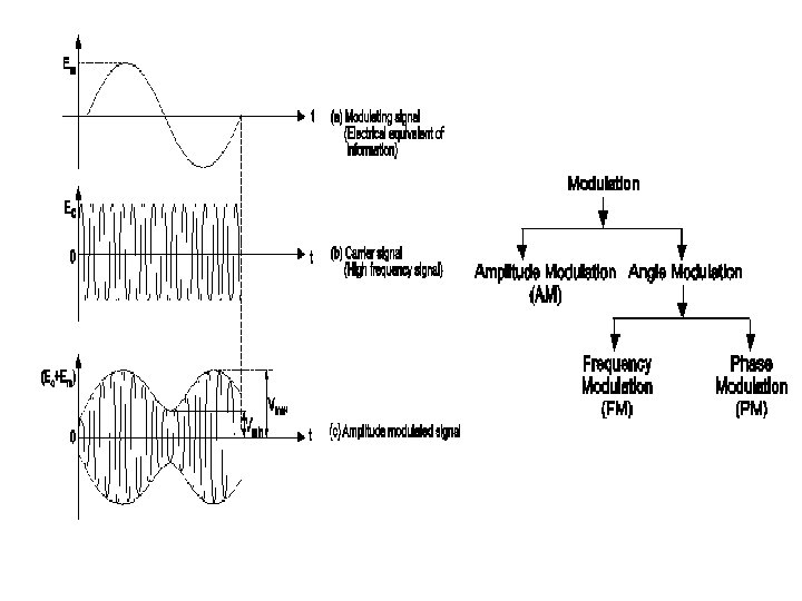
Classification of Modulation

Types AM, FM, PM Definition, Waveforms

Amplitude Modulation Definition: Amplitude modulation, is a technique of modulation in which the instantaneous amplitude of carrier signal varies in accordance with amplitude of modulating signal. While frequency and phase of carrier remains constant. Nature of Amplitude Modulated waveform shown in Fig. below.

Continued….

Modulation Index

Effect of Modulation Index on Modulated Signal

Continued….

Example Draw the AM wave for triangular and square wave modulating signal. Solution:

For square wave input.

Example 2 Draw the AM waveform for the modulation index m = 0. 75, m = 1 and m = 1. 25. (a) AM wave for m = 0. 75

Continued…

Frequency Spectrum Representation of AM wave in frequency domain is also known as frequency spectrum of AM wave. Definition: Frequency spectrum is a graph of amplitude versus frequency. The frequency spectrum of AM wave tells us about number of sidebands present in AM wave with corresponding amplitudes.

Continued……

Features of Frequency spectrum

Bandwidth Requirement The bandwidth of AM signal is defined as the frequency range from upper sideband to lower sideband frequency in frequency spectrum. BW = f. USB – f. LSB = (fc + fm) – (fc – fm) (from Fig. 2. 13) = fc + f m – f c + f m = 2 fm BW required for AM signal. Hence, bandwidth of AM signal is twice the modulating signal frequency.

Sideband Concept (DSB and SSB) DSBFC: Means double sideband full carrier as shown in Fig. 2. 13 (a). Its BW = 2 fm.

Continued… DSBSC (or DSB):

Continued… SSB:

Representation of AM Wave AM wave is represented in two ways: (i) In Time Domain (ii) In Frequency Domain

AM in Frequency Domain

Power Relations in AM Wave

Continued…

Continued….

Example 1: A modulating signal 20 sin (2 103 t) is used to modulate a carrier signal 40 sin (2 104 t). Find: (a) Modulation index (b) Percentage modulation (c) Sideband frequencies and their amplitude (d) Bandwidth of AM wave (e) Draw the frequency spectrum.

Solution: Given: Modulating signal, em = 20 sin (2 103 t) … (1) em = Em sin (2 fm t) … (2) Compare equation (1) and (2), we get Em = 20 V fm = 103 Hz = 1 k. Hz Similarly, carrier signal ec = 40 sin (2 104 t) … (3) But, ec = Ec sin (2 fc t) … (4) Compare equation (3) and (4), we get, Ec = 40 v fc = 104 Hz = 100 k. Hz (a) Modulation Index: m = = = 0. 5 (b) Percentage modulation: % modulation = = = m 100 0. 5 100 50%

(c) Sideband frequencies and their amplitude: LSB = FLSB = fc f m = 100 k. Hz 1 k. Hz = 99 k. Hz USB = FUSB = fc + f m = 100 k + 1 k. Hz = 101 k. Hz LSB amplitude = USB amplitude = = 0. 5 = 10 V (d) Bandwidth of AM BW = 2 fm = 2 1 k. Hz

AM Transmitter The functions of transmitter are: 1. To convert original information into electrical signal. 2. To amplify the weak signal. 3. To modulate the signal. 4. To increase the power level of modulated signal. 5. To transmit the signal through transmitting antenna. The AM transmitters are of two types: 1. Low level modulated transmitter. 2. High level modulated transmitter.

Low Level Modulated AM Transmitter

High Level Modulated AM Transmitter

Comparison between High Level and Low Level Modulation Sr. No. High Level Modulation place 1. Modulation takes power level. 2. Class-C amplifier are used which are highly efficient. After modulation linear amplifiers (Class A, AB or B) are used. 3. Very high efficiency. Low efficiency modulation. 4. Complex because of very high power. Easy because of low power. 5. Used in high transmitters. power at Low Level Modulation high broadcast Modulation takes power level. place than at high low level Used in TV transmitters (IF modulation method). In laboratory equipments, walkietalkies etc.

AM Modulator Circuit using BJT

Operation The transistor is normally operated in the Class-c Mode in which it is biased well beyond cut-off. • The carrier input to the base must be sufficient to drive the transistor into conduction over the part of RF cycle, during which collector current flows in the form of pulses. • The tuned circuit in the collector is tuned to resonate at the fundamental component, thus, the RF voltage at the collector is sinusoidal. • When modulating signal is applied to the steady collector voltage, changes to a slowly varying voltage given by V'cc = Vcc + Vm(t). • The modulating voltage Vm(t) is applied in series with Vcc through the low frequency transformer. • The RF bypass capacitor provides a low impedance path for the RF to ground so that negligible RF voltage is developed across the LF Transformer secondary. • The modulated output is obtained through mutual inductive coupling as shown in circuit diagram.

• The coupling prevents the 'steady' voltage from being transferred to the output, • so that Rf varies about mean value of zero shown in Fig. Input/Output waveform of AM Modulator

Advantages of AM 1. AM transmitters are not complex. 2. AM receivers are simple and easy to detect. 3. Less expensive. 4. Covers large distance. Disadvantages of AM 1. Requires large bandwidth. 2. Requires large power. 3. Gets affected due to noise. Applications of AM 1. Radio broadcasting. 2. Picture transmission in TV (VSB is used).

Angle Modulation Frequency Modulation Phase Modulation

Frequency Modulation Definition of FM: Frequency modulation is a technique of modulation in which the frequency of carrier is varied in accordance with the amplitude of modulating signal. • In FM, amplitude and phase remains constant. • Thus, the information is conveyed via. frequency changes

Modulation Index Definition: Modulation Index is defined as the ratio of frequency deviation ( ) to the modulating frequency (fm). M. I. =Frequency Deviation Modulating Frequency mf =δ fm In FM M. I. >1 Modulation Index of FM decides − (i)Bandwidth of the FM wave. (ii)Number of sidebands in FM wave.

Deviation Ratio The modulation index corresponding to maximum deviation and maximum modulating frequency is called deviation ratio. Deviation Ratio= Maximum Deviation Maximum modulating Frequency = δmax fmax In FM broadcasting the maximum value of deviation is limited to 75 k. Hz. The maximum modulating frequency is also limited to 15 k. Hz.

Percentage M. I. of FM The percentage modulation is defined as the ratio of the actual frequency deviation produced by the modulating signal to the maximum allowable frequency deviation. % M. I = Actual deviation Maximum allowable deviation

Mathematical Representation of FM (i) Modulating Signal: It may be represented as, em = Em cos mt (1) Here cos term taken for simplicity where, em = Instantaneous amplitude m = Angular velocity = 2 fm fm = Modulating frequency

(ii) Carrier Signal: Carrier may be represented as, ec = where, ec c fc = = = Ec sin ( ct + ) -----(2) Instantaneous amplitude Angular velocity 2 fc Carrier frequency Phase angle

(iii) FM Wave: Fig. Frequency Vs. Time in FM FM is nothing but a deviation of frequency. From Fig. 2. 25, it is seen that instantaneous frequency ‘f’ of the FM wave is given by, f =fc (1 + K Em cos mt) (3) where, fc =Unmodulated carrier frequency K = Proportionality constant Em cos mt =Instantaneous modulating signal (Cosine term preferred for simplicity otherwise we can use sine term also) • The maximum deviation for this particular signal will occur, when cos mt = 1 i. e. maximum. Equation (2. 26) becomes, f =fc (1 K Em) (4) f =fc K Emfc (5)

So that maximum deviation will be given by, = K Emfc (6) The instantaneous amplitude of FM signal is given by, e. FM = A sin [f( c, m)] = A sin (7) where, f( c, m)= Some function of carrier and modulating frequencies Let us write equation (2. 26) in terms of as, = c (1 + K Em cos mt) To find , must be integrated with respect to time. Thus, = dt = c (1 + K Em cos mt) dt = c (t+ KEm sin mt) m = ct + KEm c sin mt m = ct + KEmfc sin mt m

= ct + sin mt [. . . = K E m f c ] fm Substitute value of in equation (7) Thus, e. FM = A sin ( ct + sin mt )---(8) fm e. FM = A sin ( ct +mf sin mt )---(9) This is the equation of FM.

Frequency Spectrum of FM Frequency spectrum is a graph of amplitude versus frequency. The frequency spectrum of FM wave tells us about number of sideband present in the FM wave and their amplitudes. The expression for FM wave is not simple. It is complex because it is sine of sine function. Only solution is to use ‘Bessels Function’. Equation (2. 32) may be expanded as, e. FM = {A J 0 (mf) sin ct + J 1 (mf) [sin ( c + m) t − sin ( c − m) t] + J 1 (mf) [sin ( c + 2 m) t + sin ( c − 2 m) t] + J 3 (mf) [sin ( c + 3 m) t − sin ( c − 3 m) t] + J 4 (mf) [sin ( c + 4 m) t + sin ( c − 4 m) t] + } (2. 33) From this equation it is seen that the FM wave consists of: (i)Carrier (First term in equation). (ii)Infinite number of sidebands (All terms except first term are sidebands). The amplitudes of carrier and sidebands depend on ‘J’ coefficient. c = 2 fc, m = 2 fm So in place of c and m, we can use fc and fm.

Fig. : Ideal Frequency Spectrum of FM

Bandwidth of FM From frequency spectrum of FM wave shown in Fig. 2. 26, we can say that the bandwidth of FM wave is infinite. But practically, it is calculated based on how many sidebands have significant amplitudes. (i)The Simple Method to calculate the bandwidth is − BW=2 fmx Number of significant sidebands --(1) With increase in modulation index, the number of significant sidebands increases. So that bandwidth also increases. (ii)The second method to calculate bandwidth is by Carson’s rule.

Carson’s rule states that, the bandwidth of FM wave is twice the sum of deviation and highest modulating frequency. BW=2( +fmmax) (2) Highest order side band = To be found from table 2. 1 after the calculation of modulation Index m where, m = /fm e. g. If m= 20 KHZ/5 KHZ From table, for modulation index 4, highest order side band is 7 th. Therefore, the bandwidth is B. W. = 2 fm Highest order side band =2 5 k. Hz 7 =70 k. Hz

Carrier Distribution Charts: Table 2. 2: Carrier Side Band Distribution Chart for different Modulation Modulati on Index m Carri er J 0 0. 25 0. 5 1 1. 5 2 2. 4 3 4 5 5. 5 6 7 8 8. 65 0. 98 0. 94 0. 77 0. 51 0. 22 0 − 0. 26 − 0. 4 − 0. 18 0 0. 15 0. 3 0. 17 0 1 st J 1 2 nd J 2 3 rd J 3 0. 12 0. 01 0. 24 0. 03 0. 02 0. 44 0. 11 0. 06 0. 56 0. 23 0. 13 0. 58 0. 35 0. 2 0. 52 0. 43 0. 31 0. 34 0. 49 0. 43 − 0. 07 0. 36 − 0. 33 0. 05 0. 26 − 0. 34 − 0. 12 0. 11 − 0. 28 − 0. 24 − 0. 17 0 − 0. 3 − 0. 29 0. 23 − 0. 11 − 0. 24 0. 27 0. 06 4 th J 4 0. 01 0. 03 0. 06 0. 13 0. 28 0. 39 0. 4 0. 36 0. 16 − 0. 1 0. 03 Side Frequencies 5 th 6 th 7 th J 5 J 6 J 7 0. 01 0. 04 0. 13 0. 26 0. 32 0. 36 0. 35 0. 19 0. 03 0. 01 0. 05 0. 13 0. 19 0. 25 0. 34 0. 02 0. 05 0. 09 0. 13 0. 23 0. 32 0. 34 8 th J 8 0. 02 0. 03 0. 06 0. 13 0. 22 0. 28 9 th J 9 10 th 11 th 12 th J 10 J 11 J 12 0. 01 0. 02 0. 06 0. 0 3 0. 02 0. 1 0. 0 0. 13 5 0. 18 0. 0 1 0. 0 2

Effect of Modulation Index on Sidebands Modulation index 0. 5 Number of significant sideband on either side 2 of carrier 1 3 2 4 2. 5 5 4 7

Types of Frequency Modulation FM (Frequency Modulation) Narrowband FM Wideband FM (NBFM) (WBFM) [When modulation index is small] [When modulation index i large]

Comparison between Narrowband Wideband FM Sr. No. 1. Parameter 5. Modulation index Maximum deviation Range of modulating frequency Maximum modulation index Bandwidth 6. Applications 2. 3. 4. NBFM WBFM Less than or slightly greater than 1 5 k. Hz Greater than 1 20 Hz to 3 k. Hz 20 Hz to 15 k. Hz Slightly greater than 1 5 to 2500 75 k. Hz Small approximately same Large about 15 times as that of AM greater than that of BW = 2 fm NBFM. BW = 2( +fmmax) FM mobile communication Entertainment like police wireless, broadcasting (can be used ambulance, short range for high quality music ship to shore transmission) communication etc.

Representation of FM FM can be represented by two ways: 1. Time domain. 2. Frequency domain. 1. FM in Time Domain Time domain representation means continuous variation of voltage with respect to time as shown in Fig. 1 FM in Time Domain 2. FM in Frequency Domain • Frequency domain is also known as frequency spectrum. • FM in frequency domain means graph or plot of amplitude versus frequency as shown in Fig. 2. 29. Fig. 2: FM in Frequency Domain

Pre-emphasis and De-emphasis Pre and de-emphasis circuits are used only in frequency modulation. • Pre-emphasis is used at transmitter and de-emphasis at receiver. 1. Pre-emphasis • In FM, the noise has a greater effect on the higher modulating frequencies. • This effect can be reduced by increasing the value of modulation index (mf), for higher modulating frequencies. • This can be done by increasing the deviation ‘ ’ and ‘ ’ can be increased by increasing the amplitude of modulating signal at higher frequencies. Definition: The artificial boosting of higher audio modulating frequencies in accordance with prearranged response curve is called pre-emphasis. • Pre-emphasis circuit is a high pass filter as shown in Fig. 1 •

Fig. 1: Pre-emphasis Circuit

As shown in Fig. 1, AF is passed through a high-pass filter, before applying to FM modulator. • As modulating frequency (fm) increases, capacitive reactance decreases and modulating voltage goes on increasing. fm Voltage of modulating signal applied to FM modulat Boosting is done according to pre-arranged curve as shown in Fig. 2: P re-emphasis Curve

• The time constant of pre-emphasis is at 50 s in all CCIR standards. • In systems employing American FM and TV standards, networks having time constant of 75 sec are used. • The pre-emphasis is used at FM transmitter as shown in Fig. 3: FM Transmitter with Pre-emphasis

De-emphasis • De-emphasis circuit is used at FM receiver. Definition: The artificial boosting of higher modulating frequencies in the process of pre-emphasis is nullified at receiver by process called de-emphasis. • De-emphasis circuit is a low pass filter shown in Fig. 4: De-emphasis Circuit

Fig. 5: De-emphasis Curve As shown in Fig. 5, de-modulated FM is applied to the de-emphasis circuit (low pass filter) where with increase in fm, capacitive reactance Xc decreases. So that output of de-emphasis circuit also reduces • Fig. 5 shows the de-emphasis curve corresponding to a time constant 50 s. A 50 s de-emphasis corresponds to a frequency response curve that is 3 d. B down at frequency given by, f = 1/ 2πRC = 1/ 2π x 50 x 1000 = 3180 Hz

The de-emphasis circuit is used after the FM demodulator at the FM receiver shown in Fig. 6: De-emphasis Circuit in FM Receiver

Comparison between Pre-emphasis and De-emphasis Parameter 1. Circuit used Pre-emphasis High pass filter. De-emphasis Low pass filter. 2. Circuit diagram 3. Response curve Fig. 2. 36 Fig. 2. 37 Fig. 2. 38 Fig. 2. 39 4. Time constant T = RC = 50 s 5. Definition Boosting of higher frequencies Removal of higher frequencies 6. Used at FM transmitter FM receiver.

Comparison between AM and FM Parameter AM 1. Definition Amplitude of carrier is varied in accordance with amplitude of modulating signal keeping frequency and phase constant. 2. Constant parameters Frequency and phase. FM Frequency of carrier is varied in accordance with the amplitude of modulating signal keeping amplitude and phase constant. Amplitude and phase. 3. Modulated signal 4. Modulation Index m=Em/Ec m = / fm 5. Number of sidebands Only two Infinite and depends on mf. 6. Bandwidth BW = 2 fm BW = 2 ( + fm (max)) 7. Application MW, SW band broadcasting, video transmission in TV. Broadcasting FM, audio transmission in TV.

FM Generation There are two methods for generation of FM wave. Generation of FM Direct Method 1. Reactance Modulator 2. Varactor Diode Indirect Method 1. Armstrong Method

Reactance Method Fig. : Transistorized Reactance Modulator

Varactor Diode Modulator Fig. : Varactor Diode Frequency Modulator

Limitations of Direct Method of FM Generation 1. In this method, it is very difficult to get high order stability in carrier frequency because in this method the basic oscillator is not a stable oscillator, as it is controlled by the modulating signal. 2. Generally in this method we get distorted FM, due to non-linearity of the varactor diode.

FM Transmitter (Armstrong Method)

FM Generation using IC 566 Fig. : Basic Frequency Modulator using NE 566 VCO

Advantages / Disadvantages / Applications of FM Advantages of FM 1. Transmitted power remains constant. 2. FM receivers are immune to noise. 3. Good capture effect. 4. No mixing of signals. Disadvantages of FM The greatest disadvantages of FM are: 1. It uses too much spectrum space. 2. The bandwidth is wider. 3. The modulation index can be kept low to minimize the bandwidth used. 4. But reduction in M. I. reduces the noise immunity. 5. Used only at very high frequencies. Applications of FM 1. FM radio broadcasting. 2. Sound transmission in TV. 3. Police wireless.

Pulse Modulation Technique

Fig. : Carrier for Continuous Wave and Pulse Modulation

Need of Pulse Modulation • Comparing to continuous wave modulation (like AM, FM), the performance of all pulse modulation schemes except PAM in presence of noise is very good. • Due to better noise performance, it requires less power to cover large area of communication. • Due to better noise performance and requirement of less signal power, the pulse modulation is most preferred for the communication between space ships and earth.

Pulse Amplitude Modulation (PAM) Definition: • The amplitude of the pulsed carrier varies in accordance with the instantaneous value of modulating signal, is called PAM where width and position remains constant.

Generation of PAM Fig. : Generation of PAM Block diagram

Waveforms of PAM

Advantages of PAM • It is easy to generate and demodulate PAM. Disadvantages of PAM 1. Since PAM does not utilize constant amplitude pulses, output is distorted due to additive noise so that it is infrequently used. 2. Transmission bandwidth required is too large. 3. Transmitted power is not constant. Application of PAM • Used in radio telemetry for remote monitoring and sensing.

Generation of PAM Transistorized Circuit Fig. : Transistorized circuit for generation of PAM

Pulse Width Modulation (PWM) Definition: • When the width of pulsed carrier varies in accordance with the instantaneous amplitude of modulating signal, is called PWM where amplitude and position remains constant.

Generation of PWM Fig. : B. D. of generation of PWM

Waveforms of PWM

Generation of PWM using IC 555 Fig. : Generation of PWM using IC 555

. Advantages of PWM 1. More immune to noise. 2. Synchronization between transmitter and receiver is not required. 3. Possible to separate out signal from noise. Applications of PWM • PWM is used in special purpose communication systems mainly for military but is seldom used for commercial digital transmission system.

Pulse Position Modulation (PPM) Definition • When position of pulse carrier varies in accordance with the instantaneous value of modulating signal is called PPM, where width and amplitude of carrier remains constant.

Generation of PPM Fig. : Block diagram of PPM generation

Waveforms of PPM

Advantages of PPM 1. Good noise immunity. 2. Requires constant transmitter power output. Disadvantages of PPM 1. Requires synchronization between transmitter and receiver. 2. Large Bandwidth requirement. Applications of PPM 1. It is used for optical communication system where there is no multipath interference. 2. PPM is useful for narrowband FM channel allocation, with these channel characteristics in the radio control and model aircraft, boats and cars. 3. PPM is also used for military applications.

Generation of PPM using IC 555 Fig. : Generation of PPM using IC 555

Comparison of PAM, PWM and PPM Parameter PAM PWM PPM 1. Variable parameter of pulsed carrier. Amplitude Width Position 2. Bandwidth requirement Low High 3. Transmitted power Varies with amplitude of pulses Varies with variation in width Remains constant 4. Noise immunity Low High 5. Information contained in Amplitude variations Width variations Position variation 6. Output waveform

ANY QUESTION? For more detail contact us