Chapter 2 Modeling with Linear Programming sensitivity analysis

Chapter 2: Modeling with Linear Programming & sensitivity analysis Hamdy A. Taha, Operations Research: An introduction, 8 th Edition Mjdah Al Shehri 1

Mute ur call

LINEAR PROGRAMMING (LP) -In mathematics, linear programming (LP) is a technique for optimization of a linear objective function, subject to linear equality and linear inequality constraints. -Linear programming determines the way to achieve the best outcome (such as maximum profit or lowest cost) in a given mathematical model and given some list of requirements represented as linear equations. Hamdy A. Taha, Operations Research: An introduction, Prentice Hall 3

Mathematical formulation of Linear Programming model: Step 1 - Study the given situation - Find the key decision to be made - Identify the decision variables of the problem Step 2 - Formulate the objective function to be optimized Step 3 - Formulate the constraints of the problem Step 4 - Add non-negativity restrictions or constraints The objective function , the set of constraints and the non-negativity restrictions together form an LP model. Hamdy A. Taha, Operations Research: An introduction, Prentice Hall 4

TWO-VARIABLE LP MODEL EXAMPLE: “ THE GALAXY INDUSTRY PRODUCTION” • Galaxy manufactures two toy models: – Space Ray. – Zapper. • Resources are limited to – 1200 pounds of special plastic. – 40 hours of production time per week. Hamdy A. Taha, Operations Research: An introduction, Prentice Hall 5

• Marketing requirement – Total production cannot exceed 800 dozens. – Number of dozens of Space Rays cannot exceed number of dozens of Zappers by more than 450. • Technological input – Space Rays requires 2 pounds of plastic and 3 minutes of labor per dozen. – Zappers requires 1 pound of plastic and 4 minutes of labor per dozen. Hamdy A. Taha, Operations Research: An introduction, Prentice Hall 6

• Current production plan calls for: – Producing as much as possible of the more profitable product, Space Ray ($8 profit per dozen). – Use resources left over to produce Zappers ($5 profit per dozen). • The current production plan consists of: Space Rays = 550 dozens Zapper = 100 dozens Profit = 4900 dollars per week Hamdy A. Taha, Operations Research: An introduction, Prentice Hall 7

Management is seeking a production schedule that will increase the company’s profit. 8

A Linear Programming Model can provide an intelligent solution to this problem Hamdy A. Taha, Operations Research: An introduction, Prentice Hall 9

SOLUTION • Decisions variables: – X 1 = Production level of Space Rays (in dozens per week). – X 2 = Production level of Zappers (in dozens per week). • Objective Function: – Weekly profit, to be maximized Hamdy A. Taha, Operations Research: An introduction, Prentice Hall 10

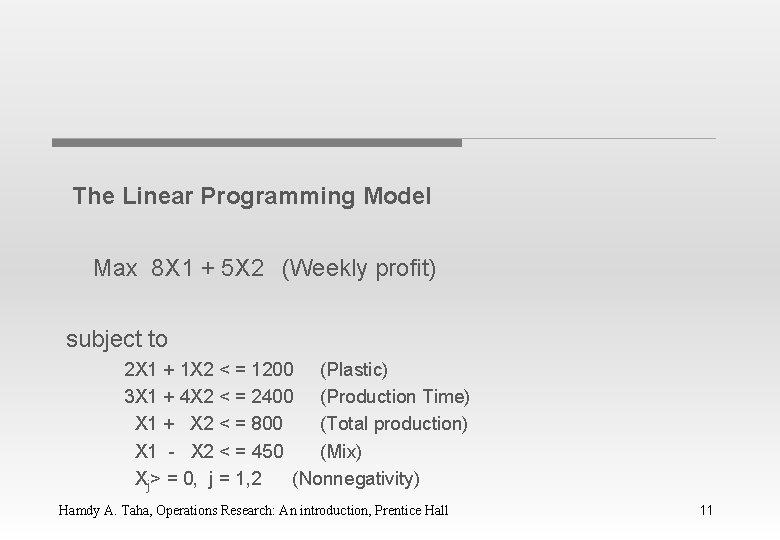
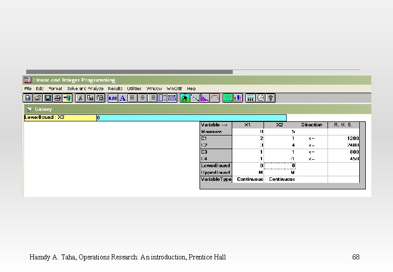
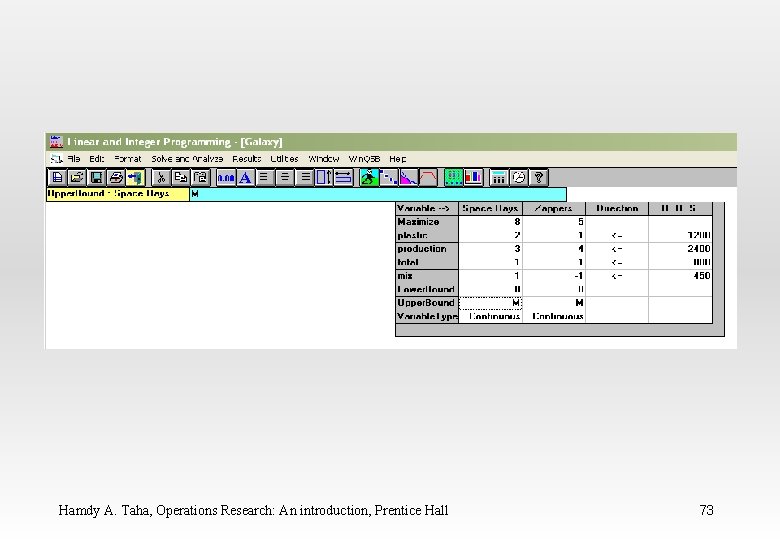
The Linear Programming Model Max 8 X 1 + 5 X 2 (Weekly profit) subject to 2 X 1 + 1 X 2 < = 1200 (Plastic) 3 X 1 + 4 X 2 < = 2400 (Production Time) X 1 + X 2 < = 800 (Total production) X 1 - X 2 < = 450 (Mix) Xj> = 0, j = 1, 2 (Nonnegativity) Hamdy A. Taha, Operations Research: An introduction, Prentice Hall 11

Feasible Solutions for Linear Programs • The set of all points that satisfy all the constraints of the model is called FEASIBLE REGION Hamdy A. Taha, Operations Research: An introduction, Prentice Hall 12

Using a graphical presentation we can represent all the constraints, the objective function, and the three types of feasible points. Hamdy A. Taha, Operations Research: An introduction, Prentice Hall 13

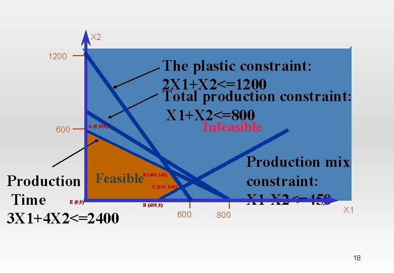
X 2 1200 The plastic constraint: The Plastic constraint 2 X 1+X 2<=1200 Total production constraint: X 1+X 2<=800 Infeasible 600 Production Feasible Time 3 X 1+4 X 2<=2400 Production mix constraint: X 1 -X 2<=450 600 800 X 1 14

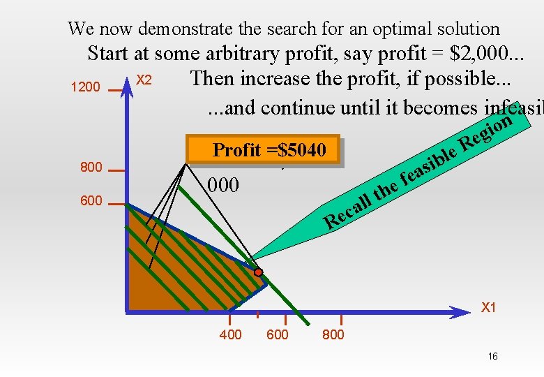
Solving Graphically for an Optimal Solution 15

We now demonstrate the search for an optimal solution Start at some arbitrary profit, say profit = $2, 000. . . X 2 Then increase the profit, if possible. . . 1200. . . and continue until it becomes infeasib 800 600 n o i eg R e l ib Profit =$5040 4, $ 2, Profit =3, s a e ef 000 h t l l a c e R X 1 400 600 800 16

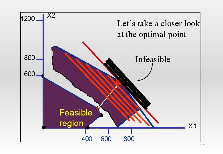
1200 X 2 Let’s take a closer look at the optimal point 800 Infeasible 600 Feasible region 400 X 1 600 800 17

X 2 1200 The plastic constraint: The Plastic constraint 2 X 1+X 2<=1200 Total production constraint: X 1+X 2<=800 600 Infeasible A (0, 600) Production Feasible Production mix constraint: X 1 -X 2<=450 B (480, 240) Time 3 X 1+4 X 2<=2400 E (0, 0) C (550, 100) D (450, 0) 600 800 X 1 18

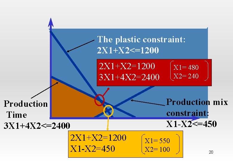
• To determine the value for X 1 and X 2 at the optimal point, the two equations of the binding constraint must be solved. Hamdy A. Taha, Operations Research: An introduction, Prentice Hall 19

The plastic constraint: 2 X 1+X 2<=1200 2 X 1+X 2=1200 3 X 1+4 X 2=2400 X 1= 480 X 2= 240 Production mix constraint: X 1 -X 2<=450 Production Time 3 X 1+4 X 2<=2400 2 X 1+X 2=1200 X 1 -X 2=450 X 1= 550 X 2= 100 20

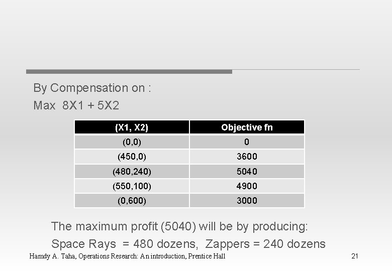
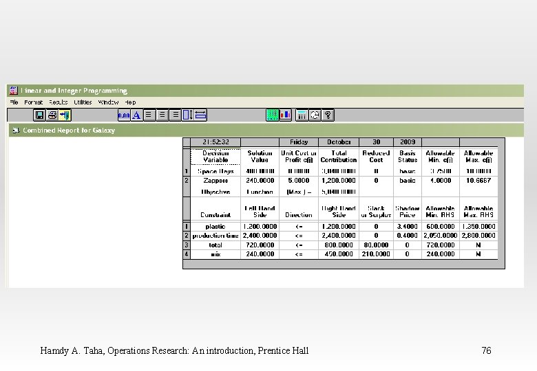
By Compensation on : Max 8 X 1 + 5 X 2 (X 1, X 2) Objective fn (0, 0) 0 (450, 0) 3600 (480, 240) 5040 (550, 100) 4900 (0, 600) 3000 The maximum profit (5040) will be by producing: Space Rays = 480 dozens, Zappers = 240 dozens Hamdy A. Taha, Operations Research: An introduction, Prentice Hall 21

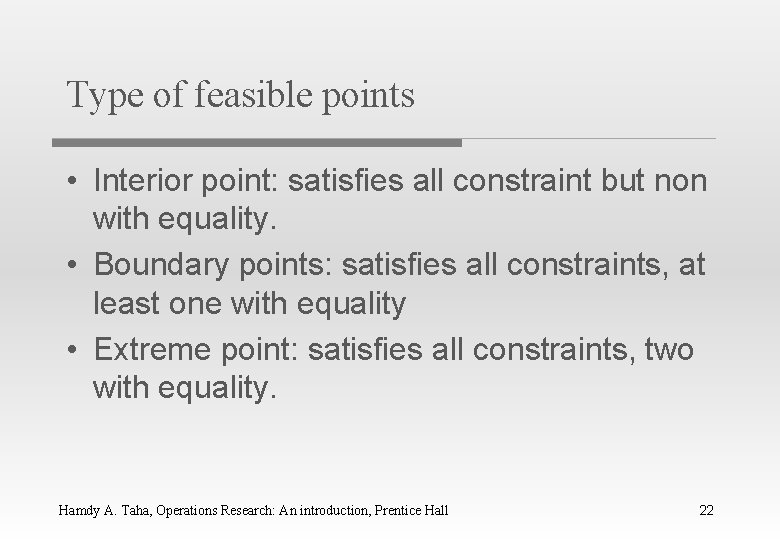
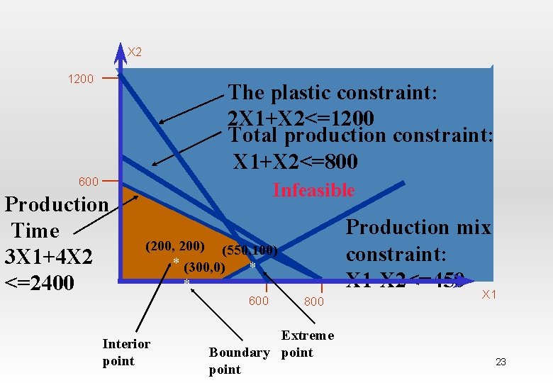
Type of feasible points • Interior point: satisfies all constraint but non with equality. • Boundary points: satisfies all constraints, at least one with equality • Extreme point: satisfies all constraints, two with equality. Hamdy A. Taha, Operations Research: An introduction, Prentice Hall 22

X 2 1200 The plastic constraint: The Plastic constraint 2 X 1+X 2<=1200 Total production constraint: X 1+X 2<=800 600 Production Time 3 X 1+4 X 2 <=2400 Infeasible Production mix constraint: X 1 -X 2<=450 (200, 200) (550, 100) * (300, 0) * * Interior point 600 800 Extreme Boundary point X 1 23

• If a linear programming has an optimal solution , an extreme point is optimal. Hamdy A. Taha, Operations Research: An introduction, Prentice Hall 24

Summery of graphical solution procedure 1 - graph constraint to find the feasible point 2 - set objective function equal to an arbitrary value so that line passes through the feasible region. 3 - move the objective function line parallel to itself until it touches the last point of the feasible region. 4 - solve for X 1 and X 2 by solving the two equation that intersect to determine this point 5 - substitute these value Prentice into Hall objective function to 25 Hamdy A. Taha, Operations Research: An introduction,

MORE EXAMPLE Hamdy A. Taha, Operations Research: An introduction, Prentice Hall 26

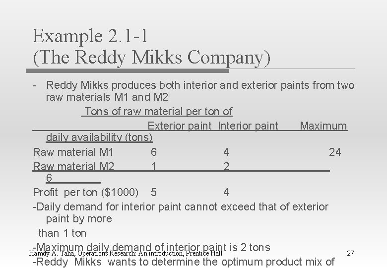
Example 2. 1 -1 (The Reddy Mikks Company) - Reddy Mikks produces both interior and exterior paints from two raw materials M 1 and M 2 Tons of raw material per ton of Exterior paint Interior paint Maximum daily availability (tons) Raw material M 1 6 4 24 Raw material M 2 1 2 6____ Profit per ton ($1000) 5 4 -Daily demand for interior paint cannot exceed that of exterior paint by more than 1 ton -Maximum daily demand of interior paint is 2 tons Hamdy A. Taha, Operations Research: An introduction, Prentice Hall 27 -Reddy Mikks wants to determine the optimum product mix of

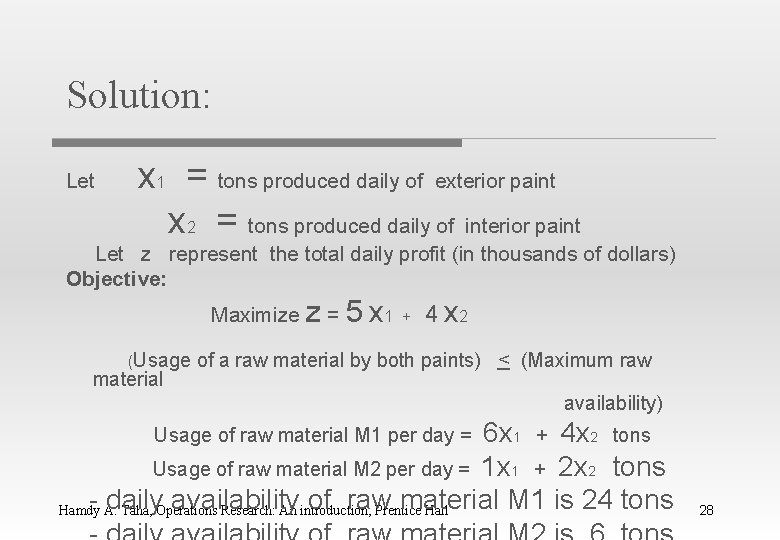
Solution: Let x 1 = tons produced daily of exterior paint x 2 = tons produced daily of interior paint Let z represent the total daily profit (in thousands of dollars) Objective: Maximize z = 5 x 1 (Usage material + 4 x 2 of a raw material by both paints) < (Maximum raw availability) 6 x 1 + 4 x 2 tons Usage of raw material M 2 per day = 1 x 1 + 2 x 2 tons - A. daily availability of raw material M 1 is 24 tons Hamdy Taha, Operations Research: An introduction, Prentice Hall Usage of raw material M 1 per day = 28

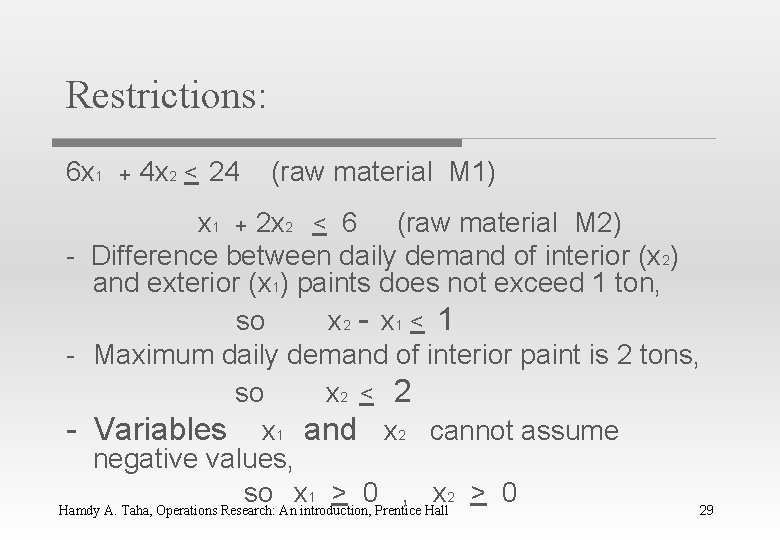
Restrictions: 6 x 1 + 4 x 2 < 24 (raw material M 1) x 1 + 2 x 2 < 6 (raw material M 2) - Difference between daily demand of interior (x 2) and exterior (x 1) paints does not exceed 1 ton, so x 2 - x 1 < 1 - Maximum daily demand of interior paint is 2 tons, so x 2 < 2 - Variables x 1 and x 2 cannot assume negative values, so x 1 > 0 , x 2 > 0 Hamdy A. Taha, Operations Research: An introduction, Prentice Hall 29

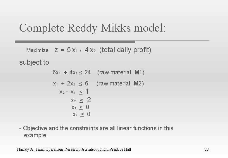
Complete Reddy Mikks model: Maximize z = 5 x 1 + 4 x 2 (total daily profit) subject to 6 x 1 + 4 x 2 < 24 (raw material M 1) x 1 + 2 x 2 < 6 (raw material M 2) x 2 - x 1 < 1 x 2 < 2 x 1 > 0 x 2 > 0 - Objective and the constraints are all linear functions in this example. Hamdy A. Taha, Operations Research: An introduction, Prentice Hall 30

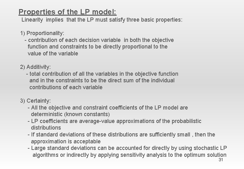
Properties of the LP model: Linearity implies that the LP must satisfy three basic properties: 1) Proportionality: - contribution of each decision variable in both the objective function and constraints to be directly proportional to the value of the variable 2) Additivity: - total contribution of all the variables in the objective function and in the constraints to be the direct sum of the individual contributions of each variable 3) Certainty: - All the objective and constraint coefficients of the LP model are deterministic (known constants) - LP coefficients are average-value approximations of the probabilistic distributions - If standard deviations of these distributions are sufficiently small , then the approximation is acceptable - Large standard deviations can be accounted for directly by using stochastic LP algorithms or indirectly by applying sensitivity analysis to the optimum solution 31

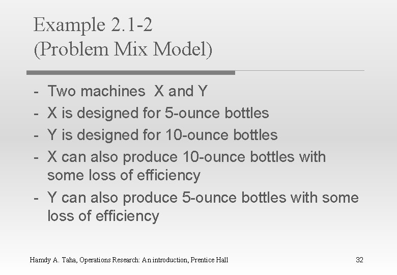
Example 2. 1 -2 (Problem Mix Model) - Two machines X and Y X is designed for 5 -ounce bottles Y is designed for 10 -ounce bottles X can also produce 10 -ounce bottles with some loss of efficiency - Y can also produce 5 -ounce bottles with some loss of efficiency Hamdy A. Taha, Operations Research: An introduction, Prentice Hall 32

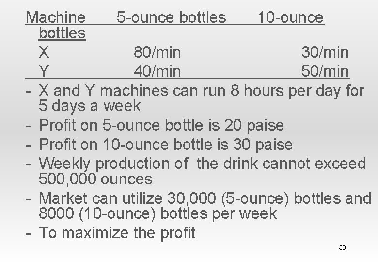
Machine 5 -ounce bottles 10 -ounce bottles X 80/min 30/min Y 40/min 50/min - X and Y machines can run 8 hours per day for 5 days a week - Profit on 5 -ounce bottle is 20 paise - Profit on 10 -ounce bottle is 30 paise - Weekly production of the drink cannot exceed 500, 000 ounces - Market can utilize 30, 000 (5 -ounce) bottles and 8000 (10 -ounce) bottles per week - To maximize the profit 33

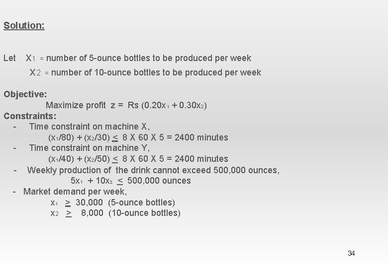
Solution: Let x 1 = number of 5 -ounce bottles to be produced per week x 2 = number of 10 -ounce bottles to be produced per week Objective: Maximize profit z = Rs (0. 20 x 1 + 0. 30 x 2) Constraints: - Time constraint on machine X, (x 1/80) + (x 2/30) < 8 X 60 X 5 = 2400 minutes - Time constraint on machine Y, (x 1/40) + (x 2/50) < 8 X 60 X 5 = 2400 minutes - Weekly production of the drink cannot exceed 500, 000 ounces, 5 x 1 + 10 x 2 < 500, 000 ounces - Market demand per week, x 1 > 30, 000 (5 -ounce bottles) x 2 > 8, 000 (10 -ounce bottles) 34

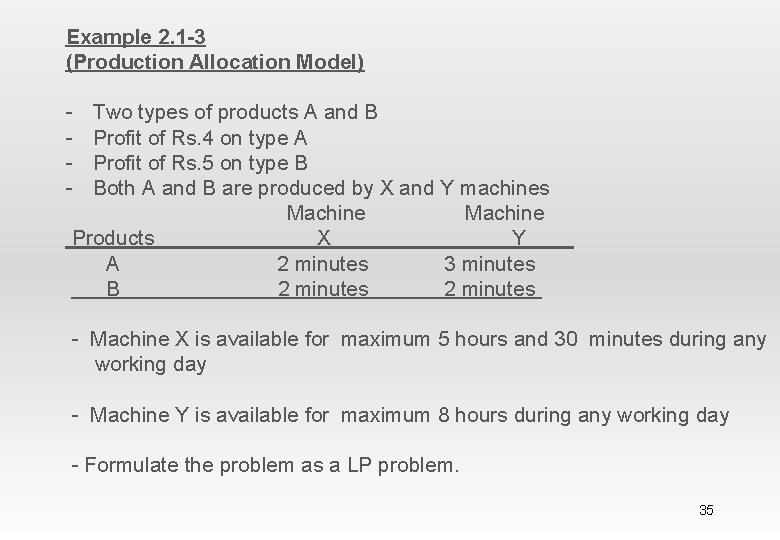
Example 2. 1 -3 (Production Allocation Model) - Two types of products A and B Profit of Rs. 4 on type A Profit of Rs. 5 on type B Both A and B are produced by X and Y machines Machine Products X Y A 2 minutes 3 minutes B 2 minutes - Machine X is available for maximum 5 hours and 30 minutes during any working day - Machine Y is available for maximum 8 hours during any working day - Formulate the problem as a LP problem. 35

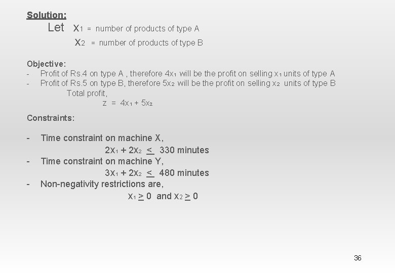
Solution: Let x 1 = number of products of type A x 2 = number of products of type B Objective: - Profit of Rs. 4 on type A , therefore 4 x 1 will be the profit on selling x 1 units of type A - Profit of Rs. 5 on type B, therefore 5 x 2 will be the profit on selling x 2 units of type B Total profit, z = 4 x 1 + 5 x 2 Constraints: - Time constraint on machine X, 2 x 1 + 2 x 2 < 330 minutes Time constraint on machine Y, 3 x 1 + 2 x 2 < 480 minutes Non-negativity restrictions are, x 1 > 0 and x 2 > 0 36

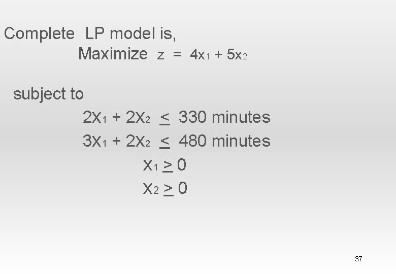
Complete LP model is, Maximize z = 4 x 1 + 5 x 2 subject to 2 x 1 + 2 x 2 < 330 minutes 3 x 1 + 2 x 2 < 480 minutes x 1 > 0 x 2 > 0 37

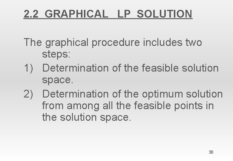
2. 2 GRAPHICAL LP SOLUTION The graphical procedure includes two steps: 1) Determination of the feasible solution space. 2) Determination of the optimum solution from among all the feasible points in the solution space. 38

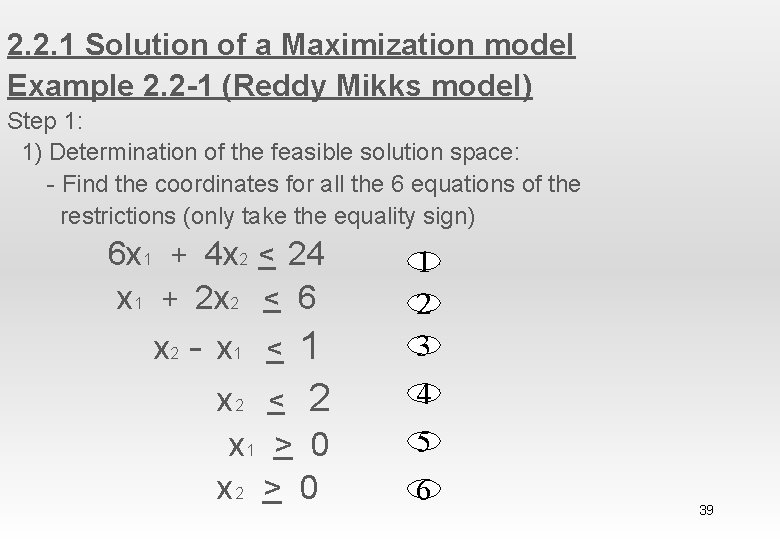
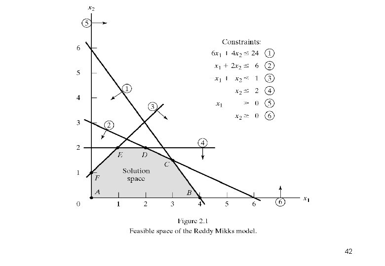
2. 2. 1 Solution of a Maximization model Example 2. 2 -1 (Reddy Mikks model) Step 1: 1) Determination of the feasible solution space: - Find the coordinates for all the 6 equations of the restrictions (only take the equality sign) 6 x 1 + 4 x 2 < 24 x 1 + 2 x 2 < 6 x 2 - x 1 < 1 x 2 < 2 x 1 > 0 x 2 > 0 1 2 3 4 5 6 39

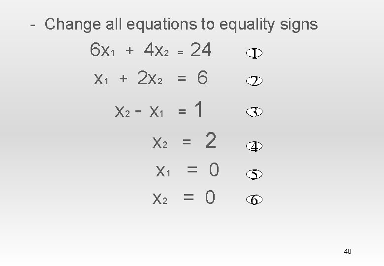
- Change all equations to equality signs 6 x 1 + 4 x 2 = 24 x 1 + 2 x 2 = 6 x 2 - x 1 = 1 x 2 = 2 x 1 = 0 x 2 = 0 1 2 3 4 5 6 40

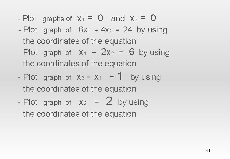
- Plot graphs of x 1 = 0 and x 2 = 0 - Plot graph of 6 x 1 + 4 x 2 = 24 by using the coordinates of the equation - Plot graph of x 1 + 2 x 2 = 6 by using the coordinates of the equation - Plot graph of x 2 - x 1 = 1 by using the coordinates of the equation - Plot graph of x 2 = 2 by using the coordinates of the equation 41

42

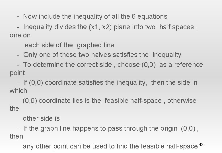
- Now include the inequality of all the 6 equations - Inequality divides the (x 1, x 2) plane into two half spaces , one on each side of the graphed line - Only one of these two halves satisfies the inequality - To determine the correct side , choose (0, 0) as a reference point - If (0, 0) coordinate satisfies the inequality, then the side in which (0, 0) coordinate lies is the feasible half-space , otherwise the other side is - If the graph line happens to pass through the origin (0, 0) , then any other point can be used to find the feasible half-space 43

Step 2: 2) Determination of the optimum solution from among all the feasible points in the solution space: - After finding out all the feasible half-spaces of all the 6 equations, feasible space is obtained by the line segments joining all the corner points A, B, C, D , E and F - Any point within or on the boundary of the solution space ABCDEF is feasible as it satisfies all the constraints - Feasible space ABCDEF consists of infinite number of feasible points 44

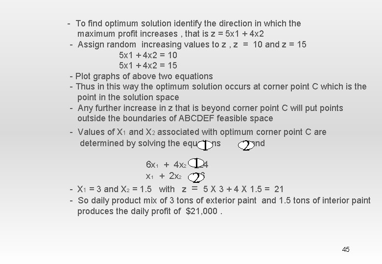
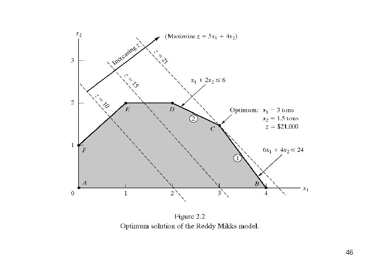
- To find optimum solution identify the direction in which the maximum profit increases , that is z = 5 x 1 + 4 x 2 - Assign random increasing values to z , z = 10 and z = 15 5 x 1 + 4 x 2 = 10 5 x 1 + 4 x 2 = 15 - Plot graphs of above two equations - Thus in this way the optimum solution occurs at corner point C which is the point in the solution space - Any further increase in z that is beyond corner point C will put points outside the boundaries of ABCDEF feasible space - Values of x 1 and x 2 associated with optimum corner point C are determined by solving the equations and 1 2 6 x 1 + 4 x 2 = 24 x 1 + 2 x 2 = 6 - x 1 = 3 and x 2 = 1. 5 with z = 5 X 3 + 4 X 1. 5 = 21 - So daily product mix of 3 tons of exterior paint and 1. 5 tons of interior paint produces the daily profit of $21, 000. 45

46

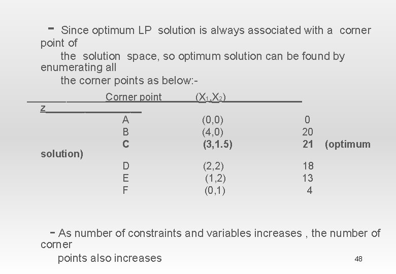
- Important characteristic of the optimum LP solution is that it is always associated with a corner point of the solution space (where two lines intersect) - This is even true if the objective function happens to be parallel to a constraint - For example if the objective function is, z = 6 x 1 + 4 x 2 - The above equation is parallel to constraint of equation 1 - So optimum occurs at either corner point B or corner point C when parallel - Actually any point on the line segment BC will be an alternative optimum - Line segment BC is totally defined by the corner points B and C 47

- Since optimum LP solution is always associated with a corner point of the solution space, so optimum solution can be found by enumerating all the corner points as below: _______Corner point z_________ A B C solution) D E F (x 1, x 2) (0, 0) (4, 0) (3, 1. 5) 0 20 21 (2, 2) (1, 2) (0, 1) 18 13 4 (optimum - As number of constraints and variables increases , the number of corner points also increases 48

2. 2. 2 Solution of a Minimization model Example 2. 2 -3 - Firm or industry has two bottling plants - One plant located at Coimbatore and other plant located at Chennai - Each plant produces three types of drinks Cocacola , Fanta and Thumps-up 49

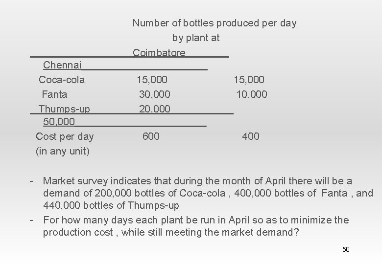
Number of bottles produced per day by plant at Coimbatore Chennai___________ Coca-cola 15, 000 Fanta 30, 000 10, 000 Thumps-up 20, 000 50, 000____________ Cost per day 600 400 (in any unit) - Market survey indicates that during the month of April there will be a demand of 200, 000 bottles of Coca-cola , 400, 000 bottles of Fanta , and 440, 000 bottles of Thumps-up - For how many days each plant be run in April so as to minimize the production cost , while still meeting the market demand? 50

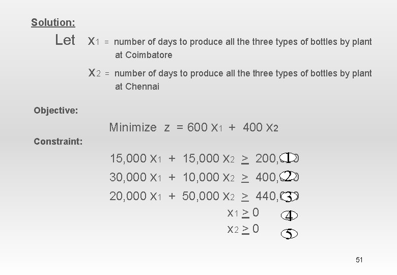
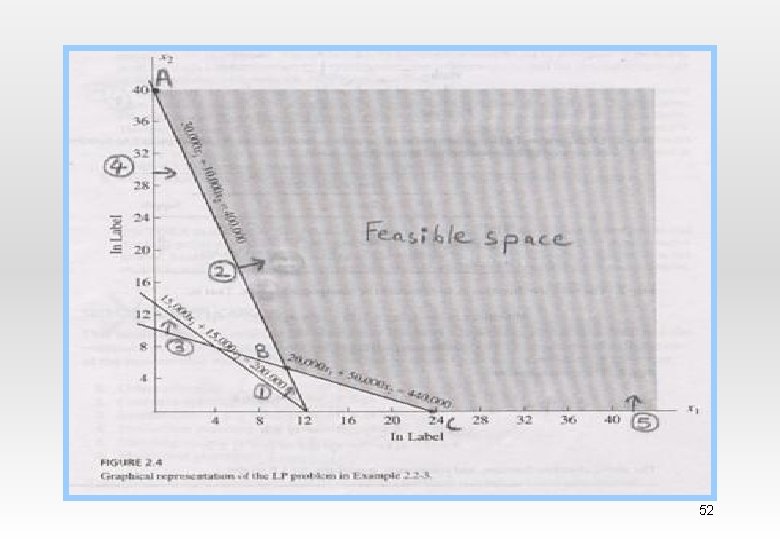
Solution: Let x 1 = number of days to produce all the three types of bottles by plant at Coimbatore x 2 = number of days to produce all the three types of bottles by plant at Chennai Objective: Minimize z = 600 x 1 + 400 x 2 Constraint: 15, 000 x 1 + 15, 000 x 2 > 200, 000 1 30, 000 x 1 + 10, 000 x 2 > 400, 000 2 20, 000 x 1 + 50, 000 x 2 > 440, 000 3 x 1 > 0 4 x 2 > 0 5 51

52

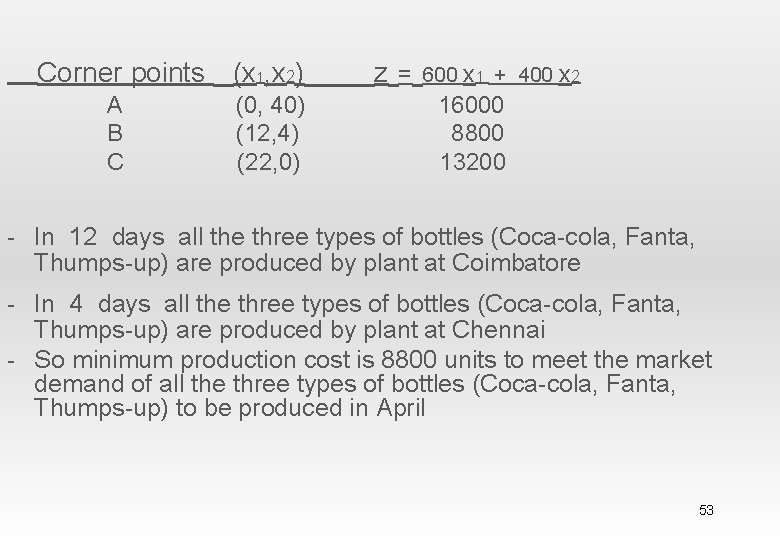
Corner points (x 1, x 2) A B C (0, 40) (12, 4) (22, 0) z= 600 x 1 + 400 x 2 16000 8800 13200 - In 12 days all the three types of bottles (Coca-cola, Fanta, Thumps-up) are produced by plant at Coimbatore - In 4 days all the three types of bottles (Coca-cola, Fanta, Thumps-up) are produced by plant at Chennai - So minimum production cost is 8800 units to meet the market demand of all the three types of bottles (Coca-cola, Fanta, Thumps-up) to be produced in April 53

Sensitivity Analysis Hamdy A. Taha, Operations Research: An introduction, Prentice Hall 54

The Role of Sensitivity Analysis of the Optimal Solution • Is the optimal solution sensitive to changes in input parameters? The effective of this change is known as “sensitivity” Hamdy A. Taha, Operations Research: An introduction, Prentice Hall 55

Sensitivity Analysis of Objective Function Coefficients. • Range of Optimality – The optimal solution will remain unchanged as long as • An objective function coefficient lies within its range of optimality • There are no changes in any other input parameters. Hamdy A. Taha, Operations Research: An introduction, Prentice Hall 56

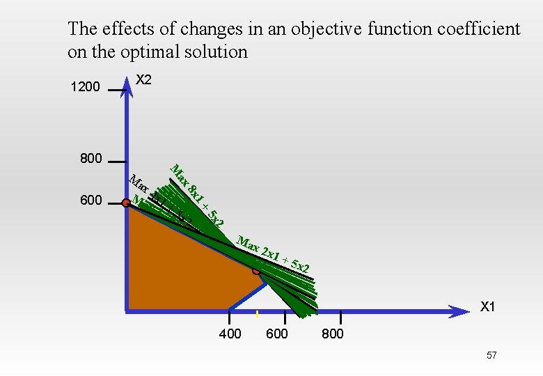
The effects of changes in an objective function coefficient on the optimal solution 1200 X 2 800 M ax Ma 4 x 1 x 3 +5. 75 x x 12 +5 1 8 x + 600 2 5 x x 2 Ma x 2 x 1+ 5 x 2 X 1 400 600 800 57

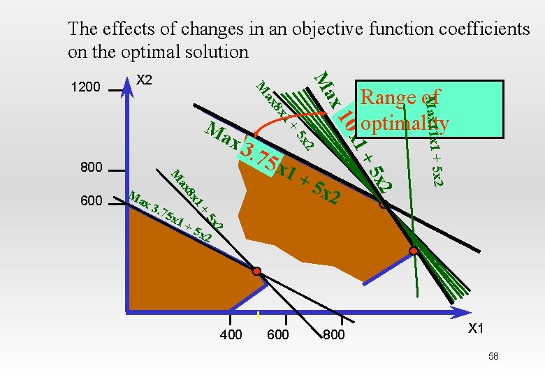
The effects of changes in an objective function coefficients on the optimal solution 5 x 2 2 x 2 5 x +5 x 2 2 5 x +5 1+ 1+ x 3. 75 x 1 8 x Ma x 100 2 x 1 ax 600 M 800 . 75 5 x x 3 1+ 8 x ax Ma Range of optimality Max 11 x 1 + x Ma X 2 M 1200 400 600 800 X 1 58

• It could be find the range of optimality for an objectives function coefficient by determining the range of values that gives a slope of the objective function line between the slopes of the binding constraints. Hamdy A. Taha, Operations Research: An introduction, Prentice Hall 59

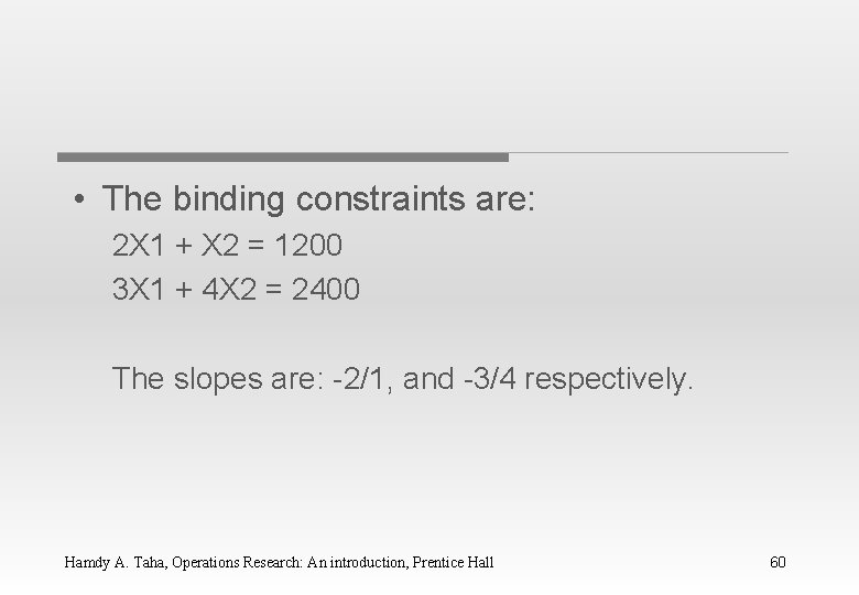
• The binding constraints are: 2 X 1 + X 2 = 1200 3 X 1 + 4 X 2 = 2400 The slopes are: -2/1, and -3/4 respectively. Hamdy A. Taha, Operations Research: An introduction, Prentice Hall 60

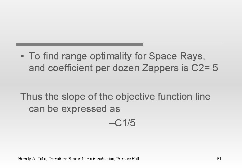
• To find range optimality for Space Rays, and coefficient per dozen Zappers is C 2= 5 Thus the slope of the objective function line can be expressed as –C 1/5 Hamdy A. Taha, Operations Research: An introduction, Prentice Hall 61

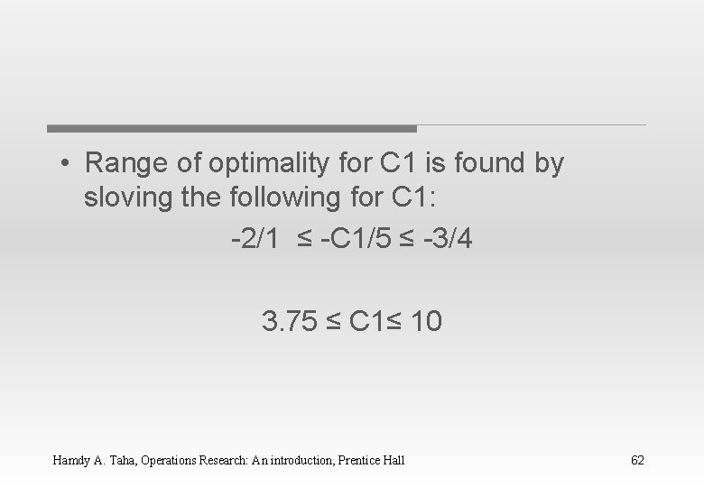
• Range of optimality for C 1 is found by sloving the following for C 1: -2/1 ≤ -C 1/5 ≤ -3/4 3. 75 ≤ C 1≤ 10 Hamdy A. Taha, Operations Research: An introduction, Prentice Hall 62

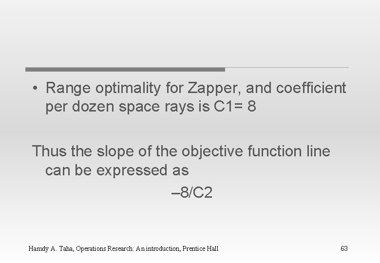
• Range optimality for Zapper, and coefficient per dozen space rays is C 1= 8 Thus the slope of the objective function line can be expressed as – 8/C 2 Hamdy A. Taha, Operations Research: An introduction, Prentice Hall 63

• Range of optimality for C 2 is found by sloving the following for C 2: -2/1 ≤ -8/C 2 ≤ -3/4 4 ≤ C 2≤ 10. 667 Hamdy A. Taha, Operations Research: An introduction, Prentice Hall 64

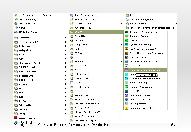
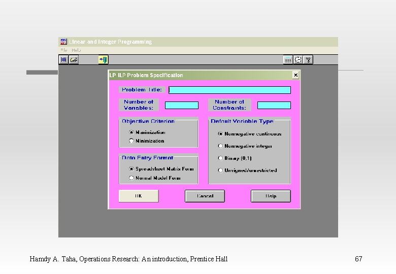
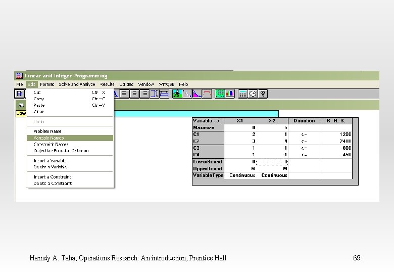
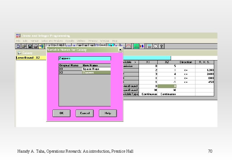
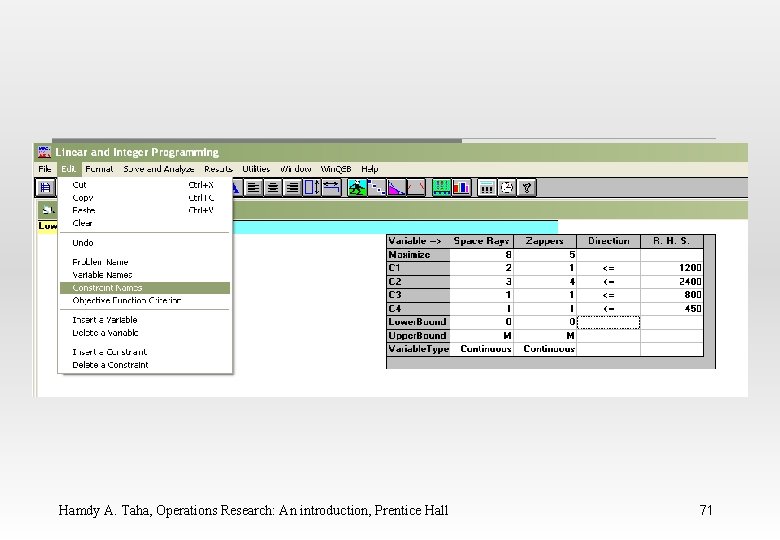
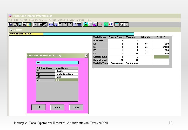
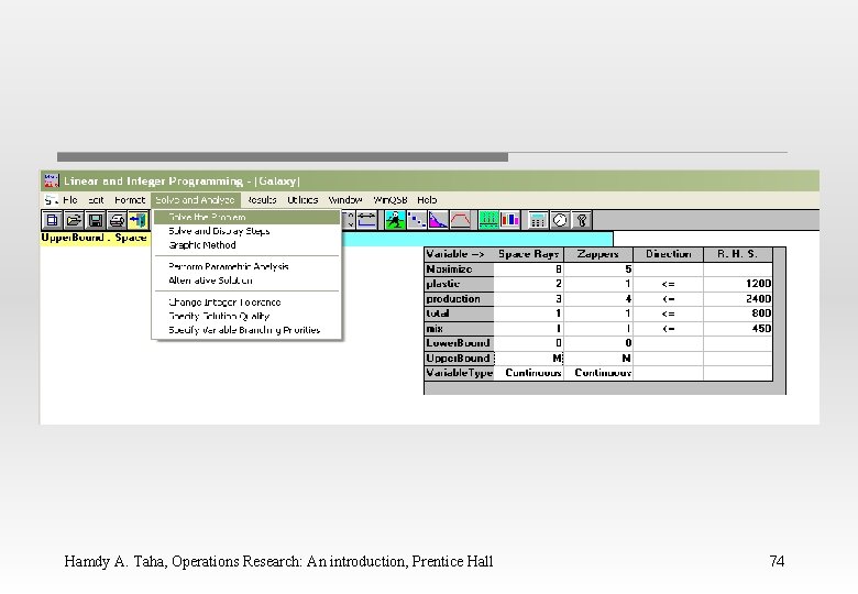
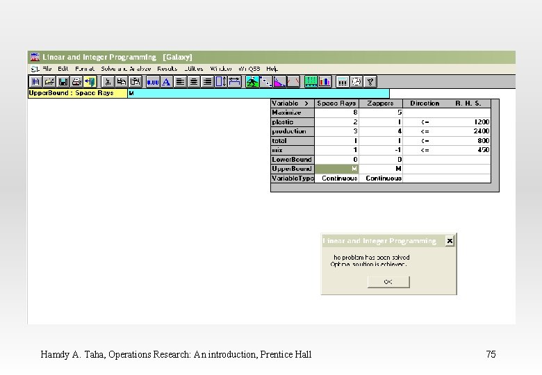
WINQSB Input Data for the Galaxy Industries Problem Hamdy A. Taha, Operations Research: An introduction, Prentice Hall 65

Hamdy A. Taha, Operations Research: An introduction, Prentice Hall 66

Hamdy A. Taha, Operations Research: An introduction, Prentice Hall 67

Hamdy A. Taha, Operations Research: An introduction, Prentice Hall 68

Hamdy A. Taha, Operations Research: An introduction, Prentice Hall 69

Hamdy A. Taha, Operations Research: An introduction, Prentice Hall 70

Hamdy A. Taha, Operations Research: An introduction, Prentice Hall 71

Hamdy A. Taha, Operations Research: An introduction, Prentice Hall 72

Hamdy A. Taha, Operations Research: An introduction, Prentice Hall 73

Hamdy A. Taha, Operations Research: An introduction, Prentice Hall 74

Hamdy A. Taha, Operations Research: An introduction, Prentice Hall 75

Hamdy A. Taha, Operations Research: An introduction, Prentice Hall 76