Chapter 2 Modeling Distributions of Data 2 1

Chapter 2: Modeling Distributions of Data

2. 1 Describing Location in a Distribution SWBAT MEASURE position using percentiles INTERPRETY cumulative frequency graphs MEASURE position using z-scores TRANSFORM data DEFINE & DESCRIBE density curves Homework

Vocabulary Percentile Z-Score(standardized score)

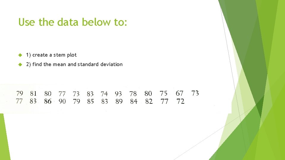
Use the data below to: 1) create a stem plot 2) find the mean and standard deviation

Percentile The percent of data that is BELOW the data you are looking at. Example. If Jenny scored an 86 on the test, how did she perform relative to the rest of the class? what was were rank? (how many scores were below hers? )

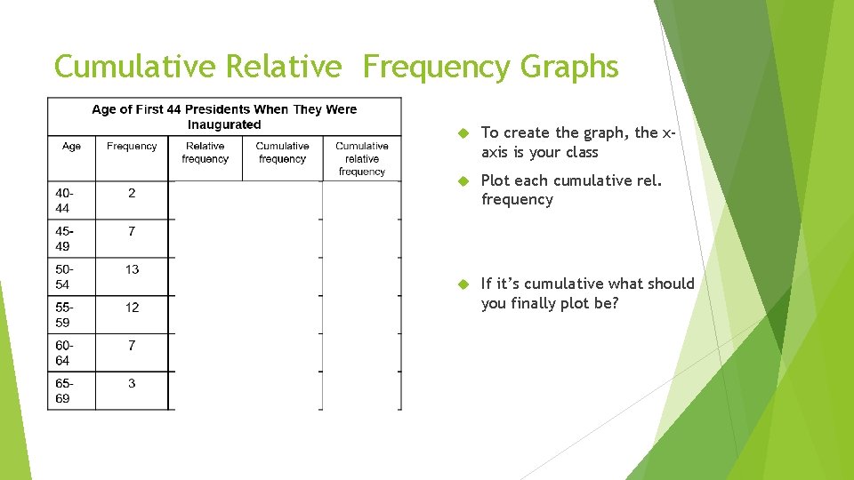
Cumulative Relative Frequency Graphs To create the graph, the xaxis is your class Plot each cumulative rel. frequency If it’s cumulative what should you finally plot be?

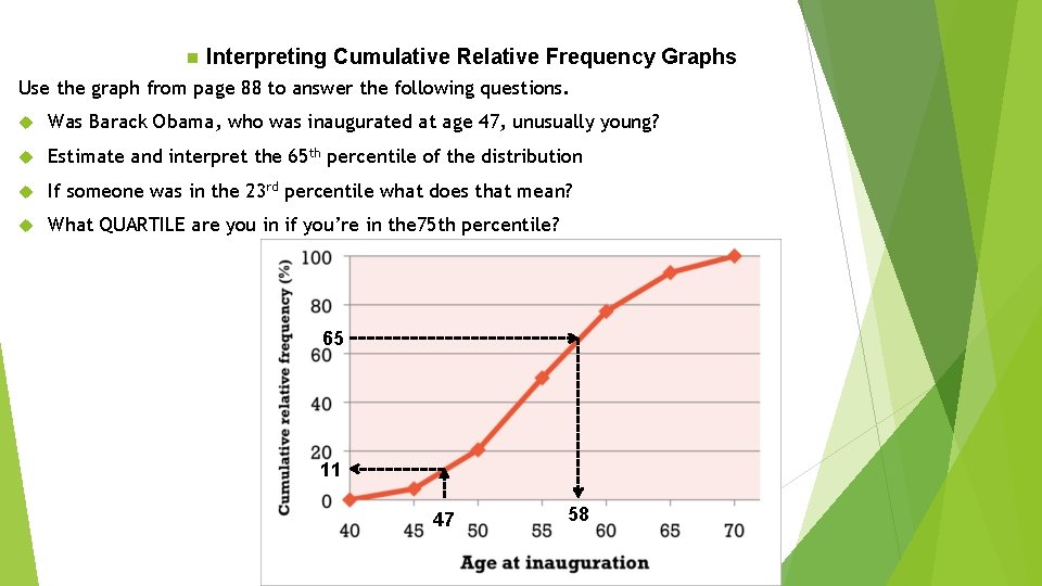
n Interpreting Cumulative Relative Frequency Graphs Use the graph from page 88 to answer the following questions. Was Barack Obama, who was inaugurated at age 47, unusually young? Estimate and interpret the 65 th percentile of the distribution If someone was in the 23 rd percentile what does that mean? What QUARTILE are you in if you’re in the 75 th percentile? 65 11 47 58

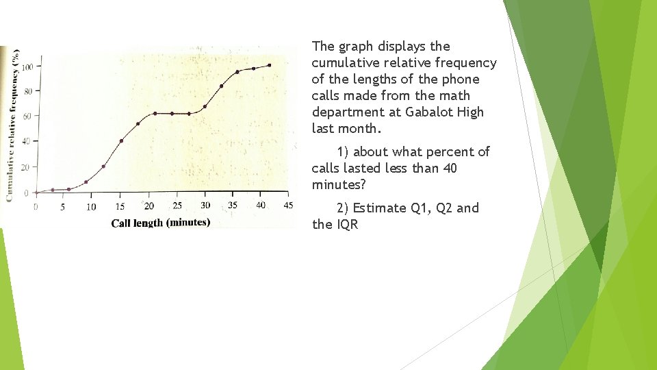
The graph displays the cumulative relative frequency of the lengths of the phone calls made from the math department at Gabalot High last month. 1) about what percent of calls lasted less than 40 minutes? 2) Estimate Q 1, Q 2 and the IQR

Mark receives a score report detailing his performance on a statewide test. On the math section, Mark earned a raw score of 39, which placed him in the 68 th percentile. This means that: a) Mark did better than 39% of the students who took the test b) Mark c) did worse than about 39% of th 3 e student who took the test. Mark did better than about 68% of student who took the test. d) Mark did worse than 68% of students who took the test e) Mark got fewer than half of the questions correct on the test.

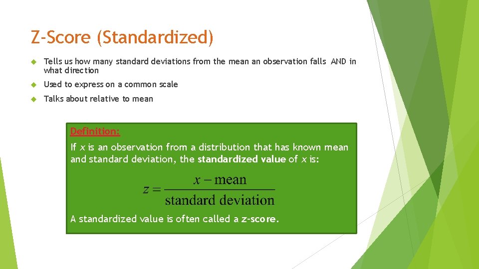
Z-Score (Standardized) Tells us how many standard deviations from the mean an observation falls AND in what direction Used to express on a common scale Talks about relative to mean Definition: If x is an observation from a distribution that has known mean and standard deviation, the standardized value of x is: A standardized value is often called a z-score.

Example Jenny earned a score of 86 on her statistics test. The class mean was 80 and the standard deviation was 6. 07. She earned a score of 82 on her chemistry test. The chemistry scores had a fairly symmetric distribution with a mean 76 and standard deviation of 4. On which test did Jenny perform better relative to the rest of her class?

Transforming Data • Transforming converts the original observations from the original units of measurements to another scale. • Transformations can affect the shape, center, and spread of a distribution. Effect of Adding (or Subtracting) a Constant Adding the same number a (either positive, zero, or negative) to each observation: • adds a to measures of center and location (mean, median, quartiles, percentiles), but • Does not change the shape of the distribution or measures of spread (range, IQR, standard deviation).

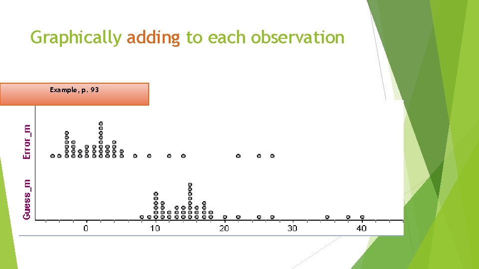
Graphically adding to each observation Example, p. 93

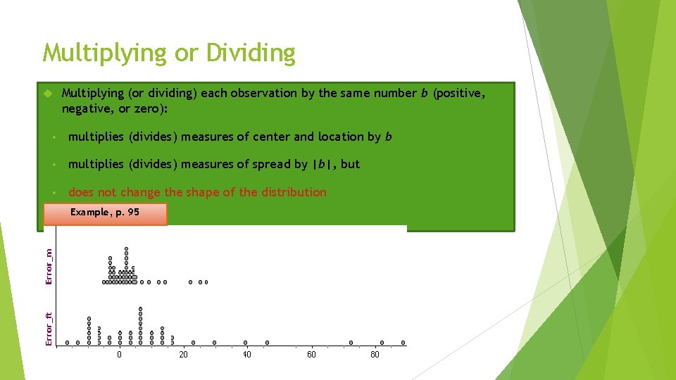
Multiplying or Dividing Multiplying (or dividing) each observation by the same number b (positive, negative, or zero): • multiplies (divides) measures of center and location by b • multiplies (divides) measures of spread by |b|, but • does not change the shape of the distribution Example, p. 95

Check your understanding 1) Suppose that you convert the class’s heights from inches to centimeters ( 1 inch – 2. 54 cm). Describe the effect this will have on the shape, center and spread of the distribution.

2. 1 Describing Location in a Distribution SWBAT MEASURE position using percentiles INTERPRETY cumulative frequency graphs MEASURE position using z-scores TRANSFORM data DEFINE & DESCRIBE density curves Homework

2. 2 Density Curves and Normal Distributions SWBAT ESTIMATE relative locations of the median and mean of a density curve APPLY 68 -95 -99. 7 rule to Normal distributions PERFORM Normal distribution calculations ASSESS Normality Homework

Vocabulary Density Curve Normal distribution Normal curve

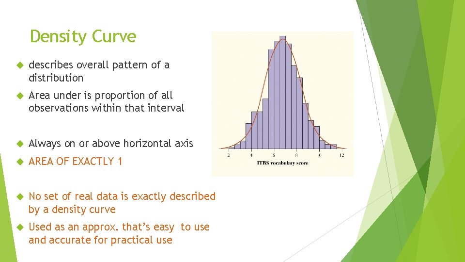
Density Curve describes overall pattern of a distribution Area under is proportion of all observations within that interval Always on or above horizontal axis AREA OF EXACTLY 1 No set of real data is exactly described by a density curve Used as an approx. that’s easy to use and accurate for practical use

Median of a density curve: Equal areas point

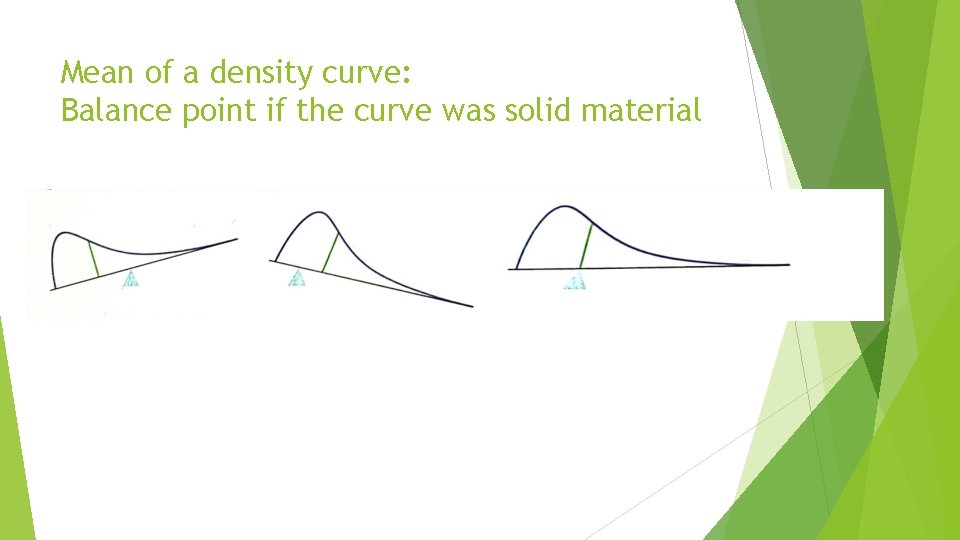
Mean of a density curve: Balance point if the curve was solid material

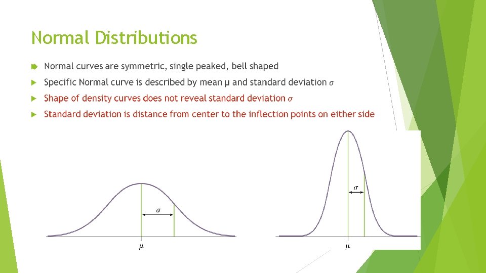
Normal Distributions

Importance of Normal distributions Good descriptions of real data such as: Test scores Repeated measurements Biological populations Good approximation of chance outcomes such as Coin tosses Slots Many statistical inference procedures are based on Normal distributions

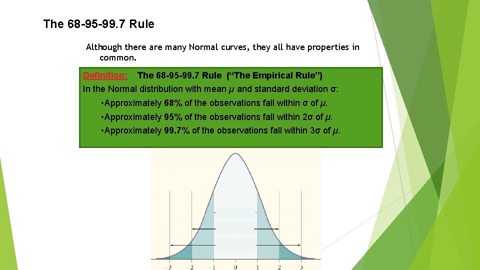
The 68 -95 -99. 7 Rule Although there are many Normal curves, they all have properties in common. Definition: The 68 -95 -99. 7 Rule (“The Empirical Rule”) In the Normal distribution with mean µ and standard deviation σ: • Approximately 68% of the observations fall within σ of µ. • Approximately 95% of the observations fall within 2σ of µ. • Approximately 99. 7% of the observations fall within 3σ of µ.

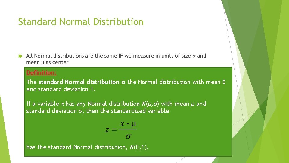
Standard Normal Distribution Definition: The standard Normal distribution is the Normal distribution with mean 0 and standard deviation 1. If a variable x has any Normal distribution N(µ, σ) with mean µ and standard deviation σ, then the standardized variable has the standard Normal distribution, N(0, 1).

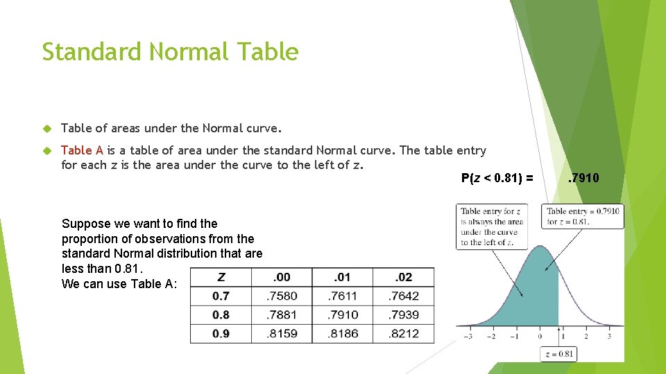
Standard Normal Table of areas under the Normal curve. Table A is a table of area under the standard Normal curve. The table entry for each z is the area under the curve to the left of z. P(z < 0. 81) = Suppose we want to find the proportion of observations from the standard Normal distribution that are less than 0. 81. We can use Table A: . 7910

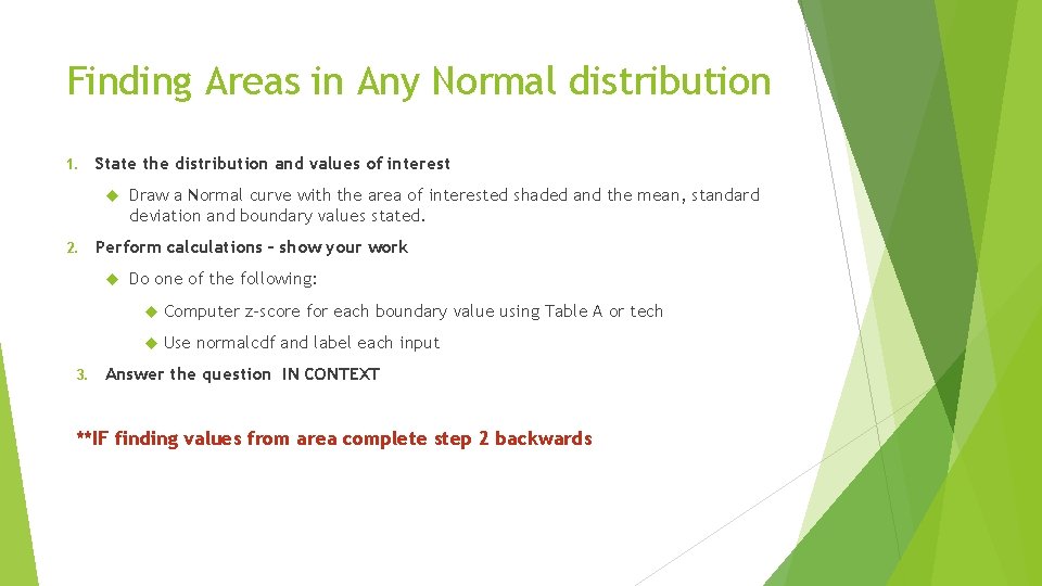
Finding Areas in Any Normal distribution 1. State the distribution and values of interest 2. Perform calculations – show your work 3. Draw a Normal curve with the area of interested shaded and the mean, standard deviation and boundary values stated. Do one of the following: Computer z-score for each boundary value using Table A or tech Use normalcdf and label each input Answer the question IN CONTEXT **IF finding values from area complete step 2 backwards

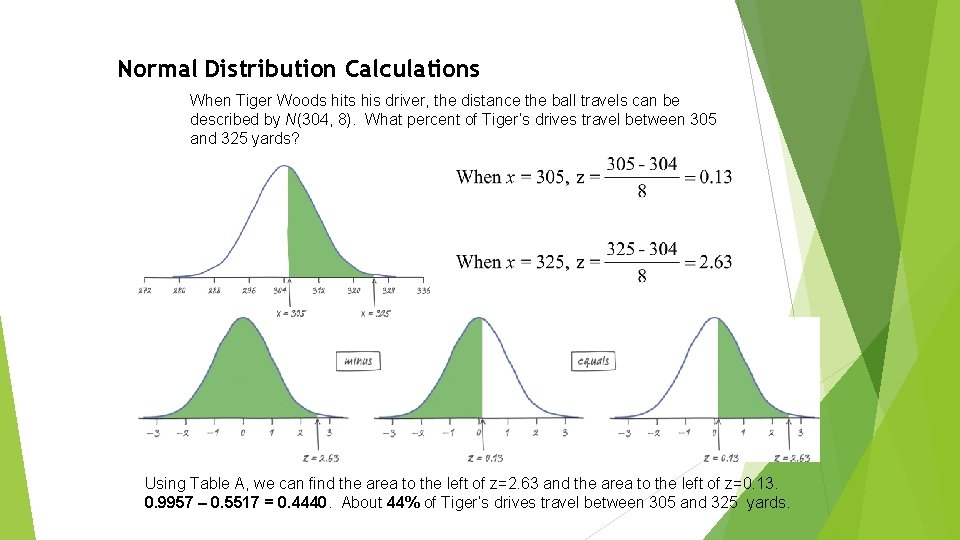
Normal Distribution Calculations When Tiger Woods hits his driver, the distance the ball travels can be described by N(304, 8). What percent of Tiger’s drives travel between 305 and 325 yards? Using Table A, we can find the area to the left of z=2. 63 and the area to the left of z=0. 13. 0. 9957 – 0. 5517 = 0. 4440. About 44% of Tiger’s drives travel between 305 and 325 yards.

Assessing Normality üPlot the data. • Make a dotplot, stemplot, or histogram and see if the graph is approximately symmetric and bell-shaped. üCheck whether the data follow the 68 -95 -99. 7 rule. • Count how many observations fall within one, two, and three standard deviations of the mean and check to see if these percents are close to the 68%, 95%, and 99. 7% targets for a Normal distribution.

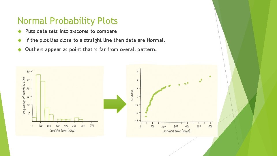
Normal Probability Plots Puts data sets into z-scores to compare If the plot lies close to a straight line then data are Normal. Outliers appear as point that is far from overall pattern.

2. 2 Density Curves and Normal Distributions SWBAT ESTIMATE relative locations of the median and mean of a density curve APPLY 68 -95 -99. 7 rule to Normal distributions PERFORM Normal distribution calculations ASSESS Normality Homework