Chapter 2 Methods for Describing Sets of Data

Describing Qualitative Data Qualitative data are nonnumeric in nature Best described by using classes 3 descriptive measures: • Class frequency – number of data points in a class • Class relative = class frequency total number of data points in the data set • Class percentage – class relative frequency x 100

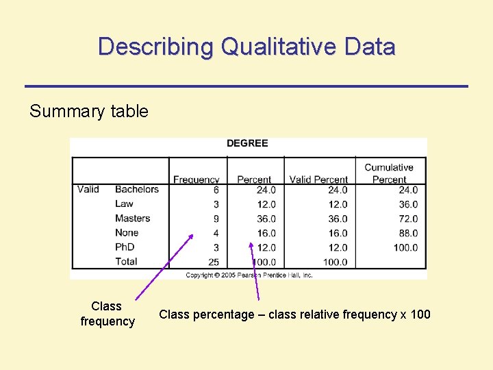
Describing Qualitative Data Summary table Class frequency Class percentage – class relative frequency x 100

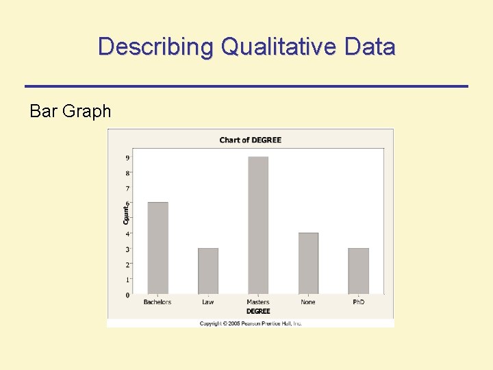
Describing Qualitative Data Bar Graph

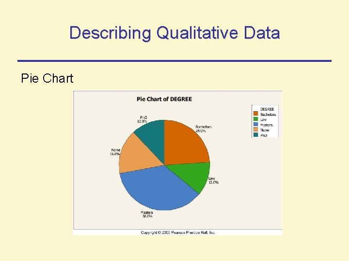
Describing Qualitative Data Pie Chart

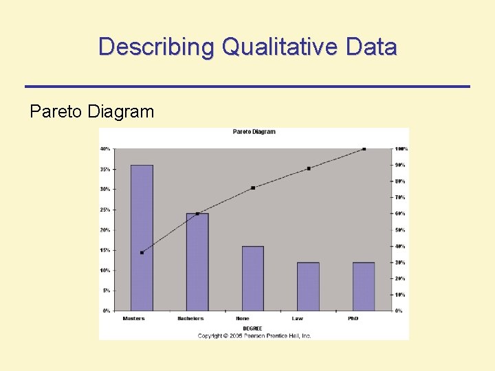
Describing Qualitative Data Pareto Diagram

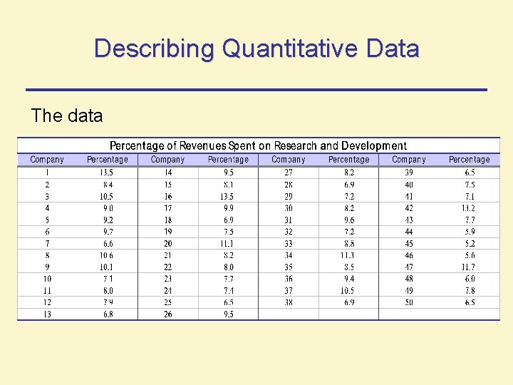
Describing Quantitative Data The data

Describing Quantitative Data For describing, summarizing, and detecting patterns in such data, we can use 3 graphical methods: • Dot plot • Stem-and-leaf display • Histogram

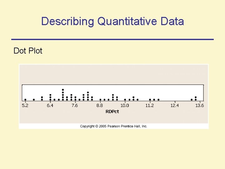
Describing Quantitative Data Dot Plot

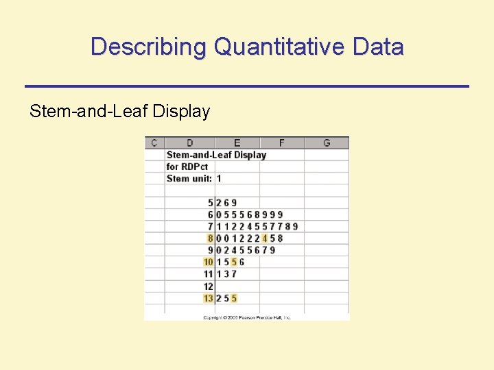
Describing Quantitative Data Stem-and-Leaf Display

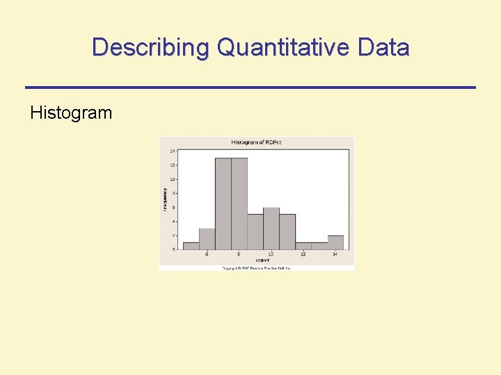
Describing Quantitative Data Histogram

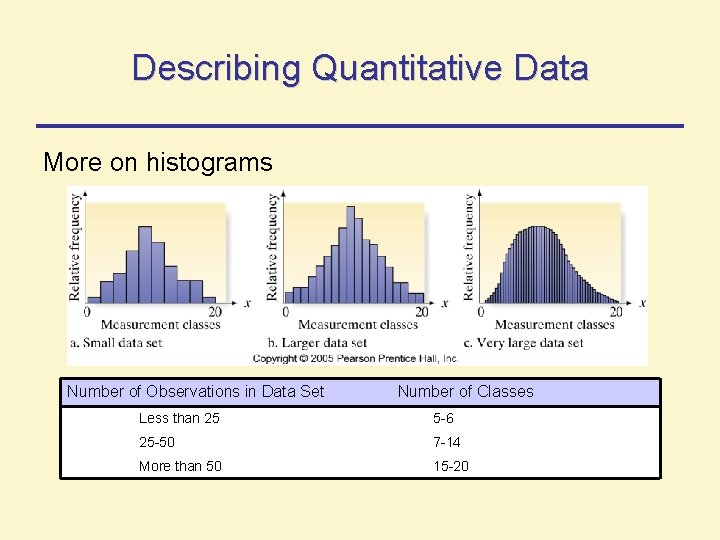
Describing Quantitative Data More on histograms Number of Observations in Data Set Number of Classes Less than 25 5 -6 25 -50 7 -14 More than 50 15 -20

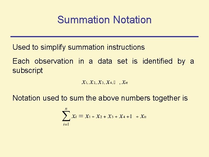
Summation Notation Used to simplify summation instructions Each observation in a data set is identified by a subscript Notation used to sum the above numbers together is

Numerical Measures of Central Tendency Central tendency – tendency of data to center about certain numerical values 3 commonly used measures of central tendency: • Mean • Median • Mode

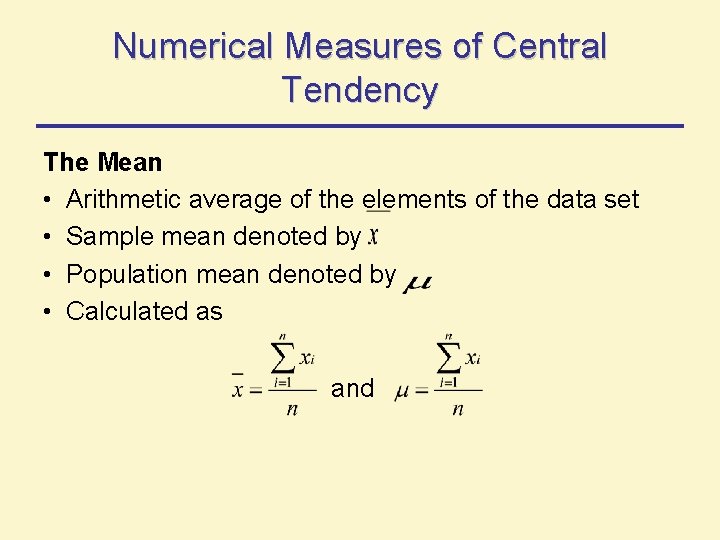
Numerical Measures of Central Tendency The Mean • Arithmetic average of the elements of the data set • Sample mean denoted by • Population mean denoted by • Calculated as and

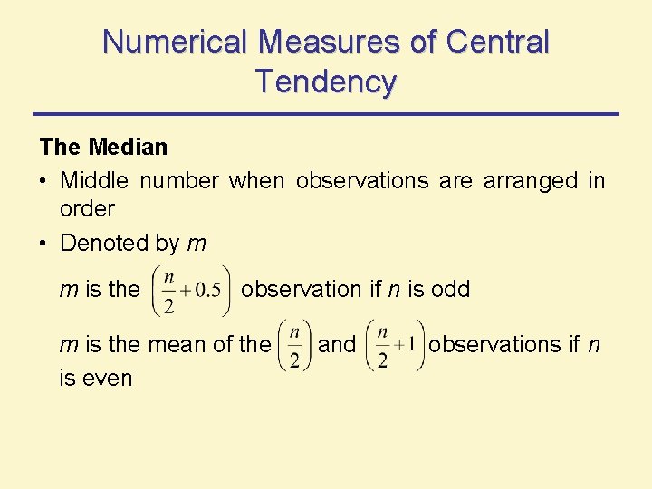
Numerical Measures of Central Tendency The Median • Middle number when observations are arranged in order • Denoted by m m is the observation if n is odd m is the mean of the is even and observations if n

Numerical Measures of Central Tendency The Mode • The most frequently occurring value in the data set • Data set can be multi-modal – have more than one mode • Data displayed in a histogram will have a modal class – the class with the largest frequency

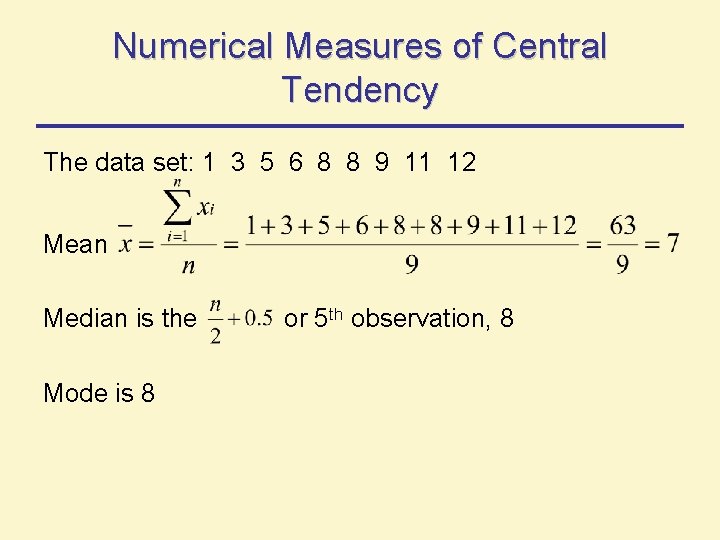
Numerical Measures of Central Tendency The data set: 1 3 5 6 8 8 9 11 12 Mean Median is the Mode is 8 or 5 th observation, 8

Numerical Measures of Variability – the spread of the data across possible values 3 commonly used measures of variability: • Range • Variance • Standard Deviation

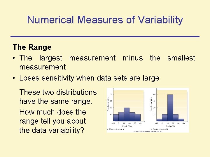
Numerical Measures of Variability The Range • The largest measurement minus the smallest measurement • Loses sensitivity when data sets are large These two distributions have the same range. How much does the range tell you about the data variability?

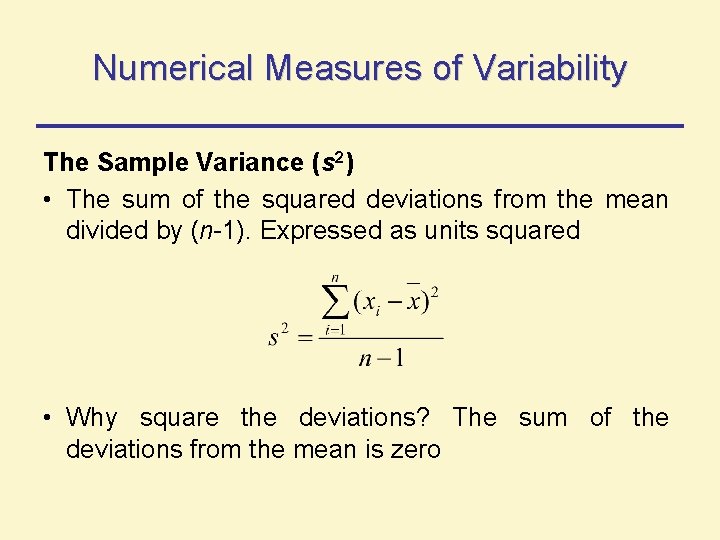
Numerical Measures of Variability The Sample Variance (s 2) • The sum of the squared deviations from the mean divided by (n-1). Expressed as units squared • Why square the deviations? The sum of the deviations from the mean is zero

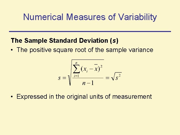
Numerical Measures of Variability The Sample Standard Deviation (s) • The positive square root of the sample variance • Expressed in the original units of measurement

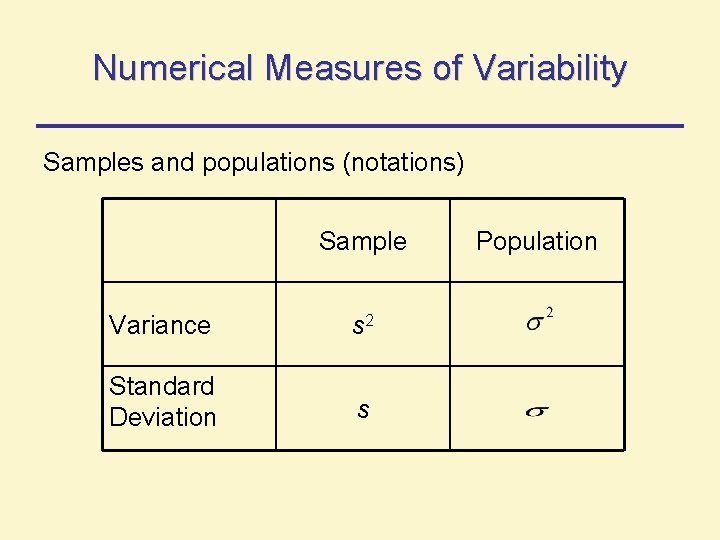
Numerical Measures of Variability Samples and populations (notations) Sample Variance s 2 Standard Deviation s Population

Numerical Measures of Relative Standing Descriptive measures of relationship measurement to the rest of the data Common measures: • Percentile ranking • z-score of a

Numerical Measures of Relative Standing Percentile rankings make use of the pth percentile For any p, the pth percentile has p% of the measures lying below it, and (100 -p)% above it The median is an example of percentiles Median is the 50 th percentile – 50% of observations lie above it and 50% lie below it

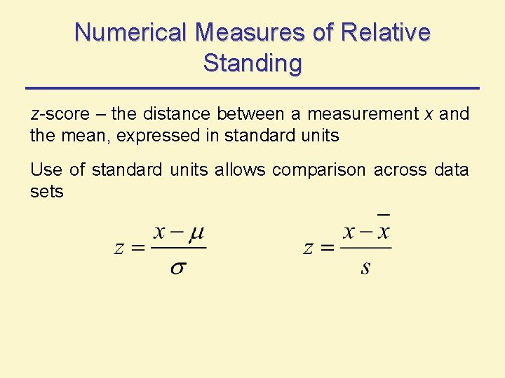
Numerical Measures of Relative Standing z-score – the distance between a measurement x and the mean, expressed in standard units Use of standard units allows comparison across data sets

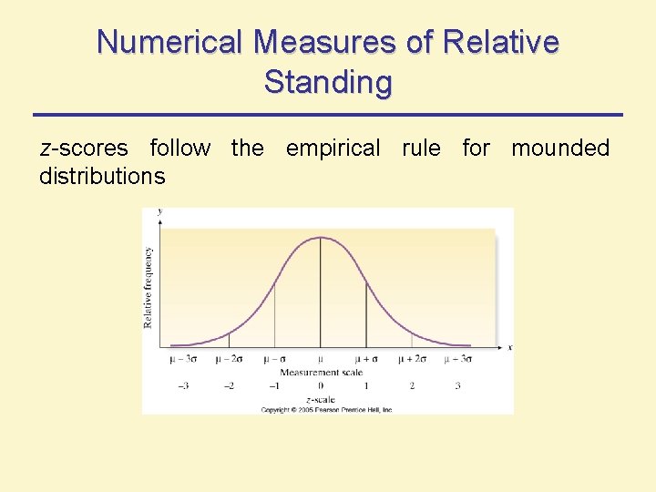
Numerical Measures of Relative Standing z-scores follow the empirical rule for mounded distributions

Methods for Detecting Outliers Outlier – an observation that is unusually large or small relative to the data values being described Causes: • Invalid measurement • Misclassified measurement • A rare (chance) event 2 detection methods: • Box Plots • z-scores

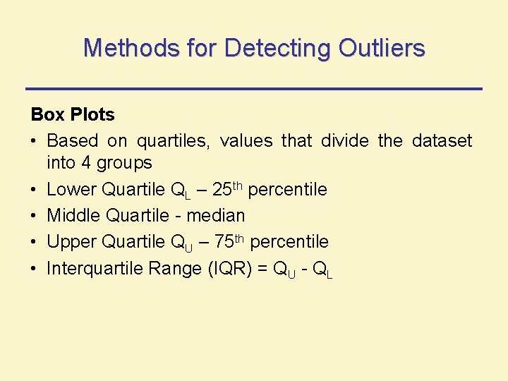
Methods for Detecting Outliers Box Plots • Based on quartiles, values that divide the dataset into 4 groups • Lower Quartile QL – 25 th percentile • Middle Quartile - median • Upper Quartile QU – 75 th percentile • Interquartile Range (IQR) = QU - QL

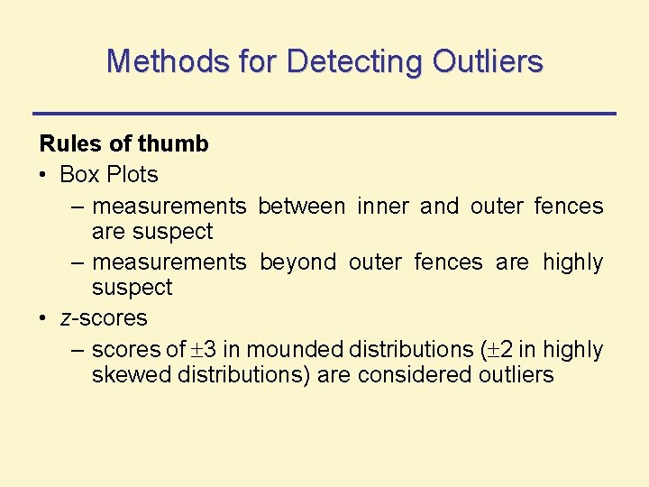
Methods for Detecting Outliers Rules of thumb • Box Plots – measurements between inner and outer fences are suspect – measurements beyond outer fences are highly suspect • z-scores – scores of 3 in mounded distributions ( 2 in highly skewed distributions) are considered outliers