Chapter 2 Linear programming 1 Introduction Many management

Chapter 2 Linear programming 1

Introduction • Many management decisions involve trying to make the most effective use of an organization’s resources. • Resources typically include machinery, labor, money, time, warehouse space, or raw materials. • Linear programming (LP) is a widely used mathematical technique designed to help managers in planning and decision making relative to resource allocation. • Despite the name, linear programming, and the more general category of techniques called “mathematical programming”, have very little to do with computer programming. • In the world of Operations Research, programming refers to modeling and solving a problem mathematically. • Computer programming has, however, played an important role in the advancement and use of LP to solve real-life LP problems 2

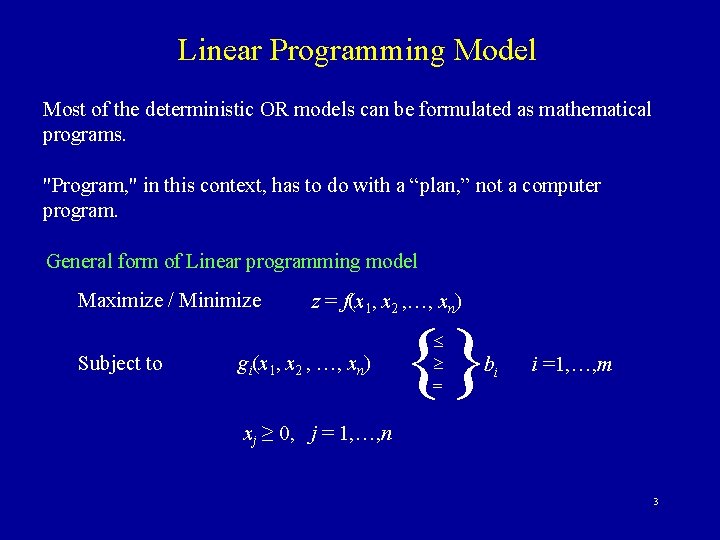
Linear Programming Model Most of the deterministic OR models can be formulated as mathematical programs. "Program, " in this context, has to do with a “plan, ” not a computer program. General form of Linear programming model Maximize / Minimize Subject to z = f(x 1, x 2 , …, xn) gi(x 1, x 2 , …, xn) {} = bi i =1, …, m xj ≥ 0, j = 1, …, n 3

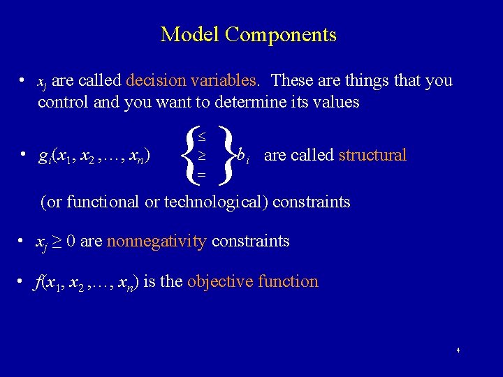
Model Components • xj are called decision variables. These are things that you control and you want to determine its values • gi(x 1, x 2 , …, xn) {} = bi are called structural (or functional or technological) constraints • xj ≥ 0 are nonnegativity constraints • f(x 1, x 2 , …, xn) is the objective function 4

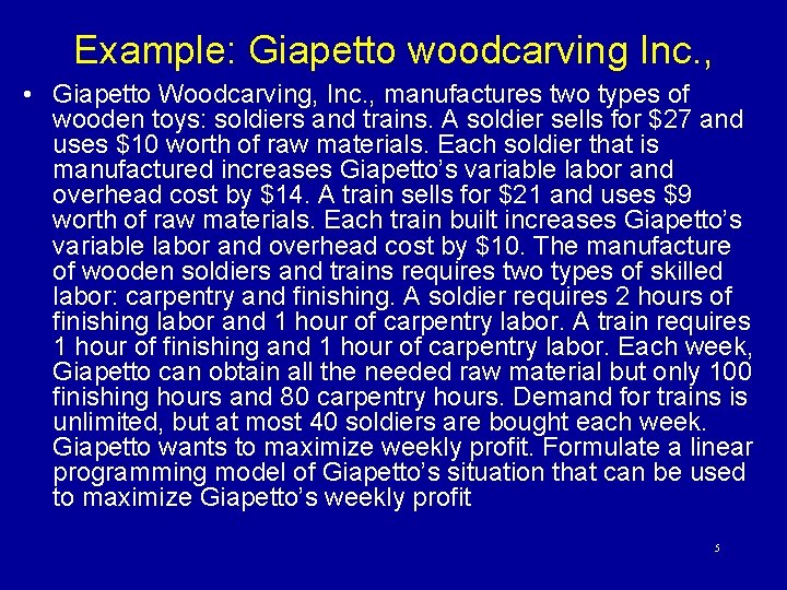
Example: Giapetto woodcarving Inc. , • Giapetto Woodcarving, Inc. , manufactures two types of wooden toys: soldiers and trains. A soldier sells for $27 and uses $10 worth of raw materials. Each soldier that is manufactured increases Giapetto’s variable labor and overhead cost by $14. A train sells for $21 and uses $9 worth of raw materials. Each train built increases Giapetto’s variable labor and overhead cost by $10. The manufacture of wooden soldiers and trains requires two types of skilled labor: carpentry and finishing. A soldier requires 2 hours of finishing labor and 1 hour of carpentry labor. A train requires 1 hour of finishing and 1 hour of carpentry labor. Each week, Giapetto can obtain all the needed raw material but only 100 finishing hours and 80 carpentry hours. Demand for trains is unlimited, but at most 40 soldiers are bought each week. Giapetto wants to maximize weekly profit. Formulate a linear programming model of Giapetto’s situation that can be used to maximize Giapetto’s weekly profit 5

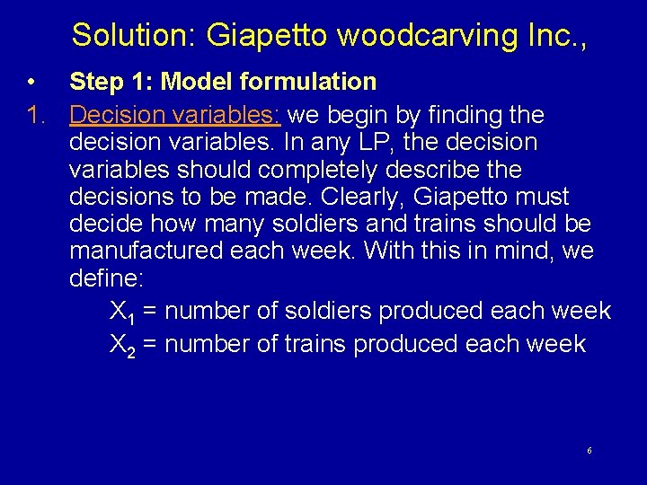
Solution: Giapetto woodcarving Inc. , • Step 1: Model formulation 1. Decision variables: we begin by finding the decision variables. In any LP, the decision variables should completely describe the decisions to be made. Clearly, Giapetto must decide how many soldiers and trains should be manufactured each week. With this in mind, we define: X 1 = number of soldiers produced each week X 2 = number of trains produced each week 6

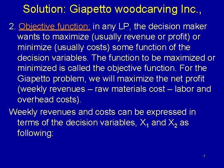
Solution: Giapetto woodcarving Inc. , 2. Objective function: in any LP, the decision maker wants to maximize (usually revenue or profit) or minimize (usually costs) some function of the decision variables. The function to be maximized or minimized is called the objective function. For the Giapetto problem, we will maximize the net profit (weekly revenues – raw materials cost – labor and overhead costs). Weekly revenues and costs can be expressed in terms of the decision variables, X 1 and X 2 as following: 7

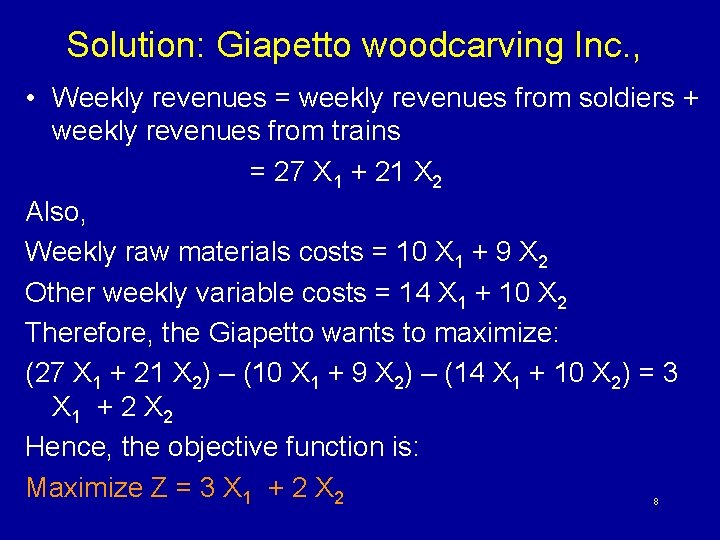
Solution: Giapetto woodcarving Inc. , • Weekly revenues = weekly revenues from soldiers + weekly revenues from trains = 27 X 1 + 21 X 2 Also, Weekly raw materials costs = 10 X 1 + 9 X 2 Other weekly variable costs = 14 X 1 + 10 X 2 Therefore, the Giapetto wants to maximize: (27 X 1 + 21 X 2) – (10 X 1 + 9 X 2) – (14 X 1 + 10 X 2) = 3 X 1 + 2 X 2 Hence, the objective function is: Maximize Z = 3 X 1 + 2 X 2 8

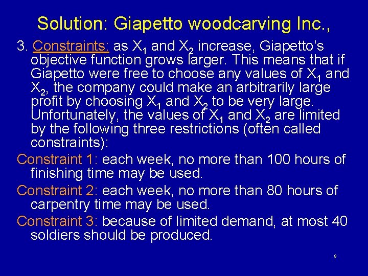
Solution: Giapetto woodcarving Inc. , 3. Constraints: as X 1 and X 2 increase, Giapetto’s objective function grows larger. This means that if Giapetto were free to choose any values of X 1 and X 2, the company could make an arbitrarily large profit by choosing X 1 and X 2 to be very large. Unfortunately, the values of X 1 and X 2 are limited by the following three restrictions (often called constraints): Constraint 1: each week, no more than 100 hours of finishing time may be used. Constraint 2: each week, no more than 80 hours of carpentry time may be used. Constraint 3: because of limited demand, at most 40 soldiers should be produced. 9

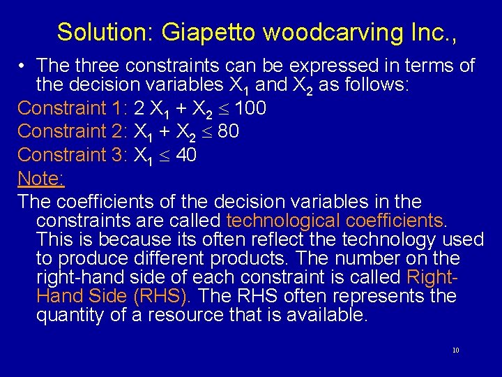
Solution: Giapetto woodcarving Inc. , • The three constraints can be expressed in terms of the decision variables X 1 and X 2 as follows: Constraint 1: 2 X 1 + X 2 100 Constraint 2: X 1 + X 2 80 Constraint 3: X 1 40 Note: The coefficients of the decision variables in the constraints are called technological coefficients. This is because its often reflect the technology used to produce different products. The number on the right-hand side of each constraint is called Right. Hand Side (RHS). The RHS often represents the quantity of a resource that is available. 10

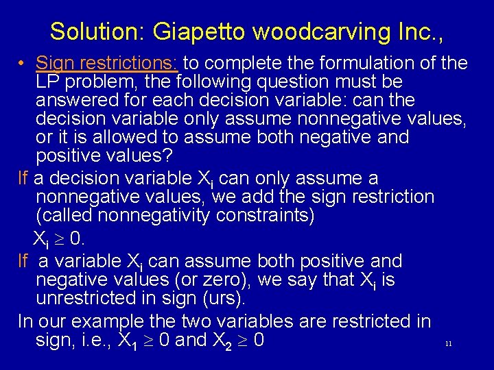
Solution: Giapetto woodcarving Inc. , • Sign restrictions: to complete the formulation of the LP problem, the following question must be answered for each decision variable: can the decision variable only assume nonnegative values, or it is allowed to assume both negative and positive values? If a decision variable Xi can only assume a nonnegative values, we add the sign restriction (called nonnegativity constraints) Xi 0. If a variable Xi can assume both positive and negative values (or zero), we say that Xi is unrestricted in sign (urs). In our example the two variables are restricted in sign, i. e. , X 1 0 and X 2 0 11

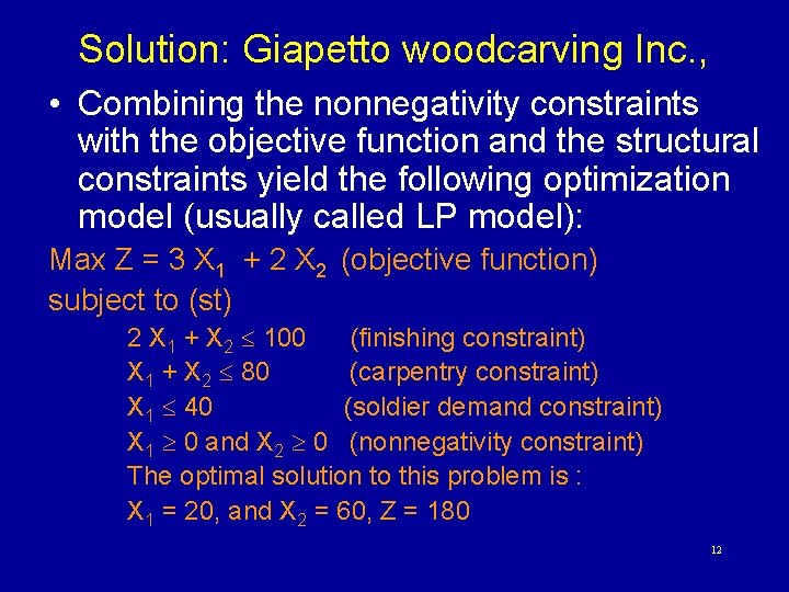
Solution: Giapetto woodcarving Inc. , • Combining the nonnegativity constraints with the objective function and the structural constraints yield the following optimization model (usually called LP model): Max Z = 3 X 1 + 2 X 2 (objective function) subject to (st) 2 X 1 + X 2 100 (finishing constraint) X 1 + X 2 80 (carpentry constraint) X 1 40 (soldier demand constraint) X 1 0 and X 2 0 (nonnegativity constraint) The optimal solution to this problem is : X 1 = 20, and X 2 = 60, Z = 180 12

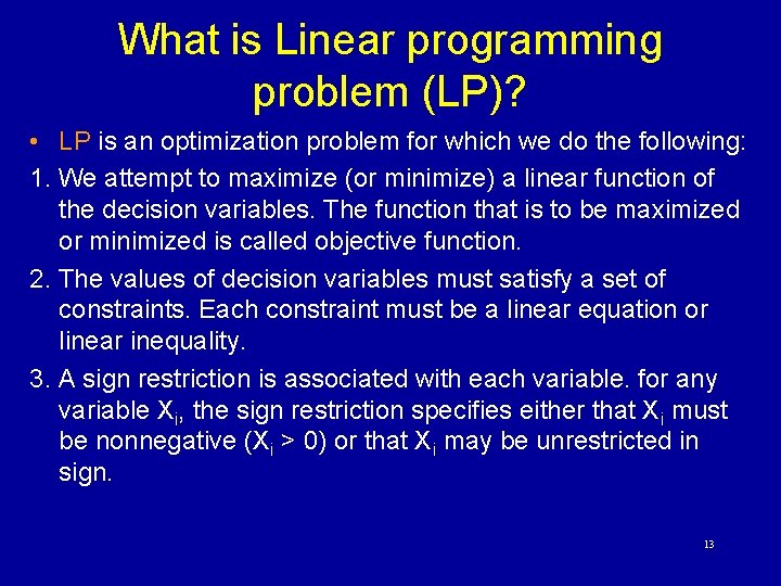
What is Linear programming problem (LP)? • LP is an optimization problem for which we do the following: 1. We attempt to maximize (or minimize) a linear function of the decision variables. The function that is to be maximized or minimized is called objective function. 2. The values of decision variables must satisfy a set of constraints. Each constraint must be a linear equation or linear inequality. 3. A sign restriction is associated with each variable. for any variable Xi, the sign restriction specifies either that Xi must be nonnegative (Xi > 0) or that Xi may be unrestricted in sign. 13

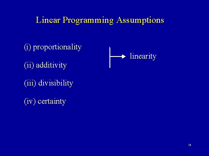
Linear Programming Assumptions (i) proportionality linearity (ii) additivity (iii) divisibility (iv) certainty 14

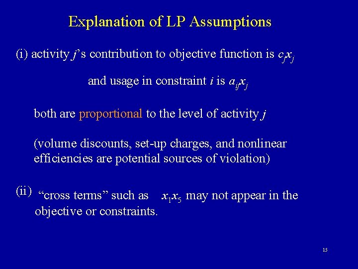
Explanation of LP Assumptions (i) activity j’s contribution to objective function is cjxj and usage in constraint i is aijxj both are proportional to the level of activity j (volume discounts, set-up charges, and nonlinear efficiencies are potential sources of violation) (ii) “cross terms” such as x x may not appear in the 1 5 objective or constraints. 15

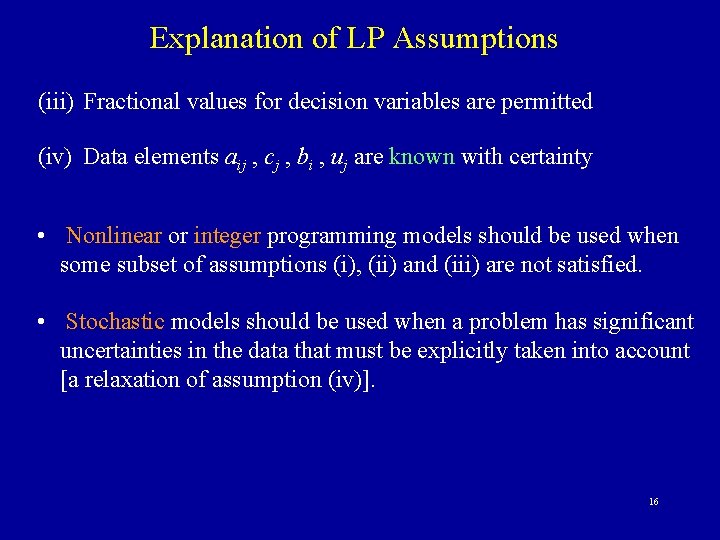
Explanation of LP Assumptions (iii) Fractional values for decision variables are permitted (iv) Data elements aij , cj , bi , uj are known with certainty • Nonlinear or integer programming models should be used when some subset of assumptions (i), (ii) and (iii) are not satisfied. • Stochastic models should be used when a problem has significant uncertainties in the data that must be explicitly taken into account [a relaxation of assumption (iv)]. 16

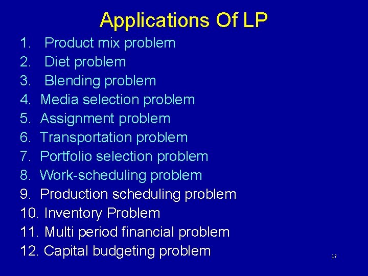
Applications Of LP 1. Product mix problem 2. Diet problem 3. Blending problem 4. Media selection problem 5. Assignment problem 6. Transportation problem 7. Portfolio selection problem 8. Work-scheduling problem 9. Production scheduling problem 10. Inventory Problem 11. Multi period financial problem 12. Capital budgeting problem 17

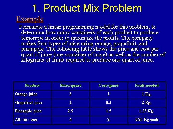
1. Product Mix Problem Example Formulate a linear programming model for this problem, to determine how many containers of each product to produce tomorrow in order to maximize the profits. The company makes four types of juice using orange, grapefruit, and pineapple. The following table shows the price and cost per quart of juice (one container of juice) as well as the number of kilograms of fruits required to produce one quart of juice. Product Price/quart Cost/quart Fruit needed Orange juice 3 1 1 Kg. Grapefruit juice 2 0. 5 2 Kg. Pineapple juice 2. 5 1. 25 Kg. 4 2 18 0. 25 Kg each All –in - one

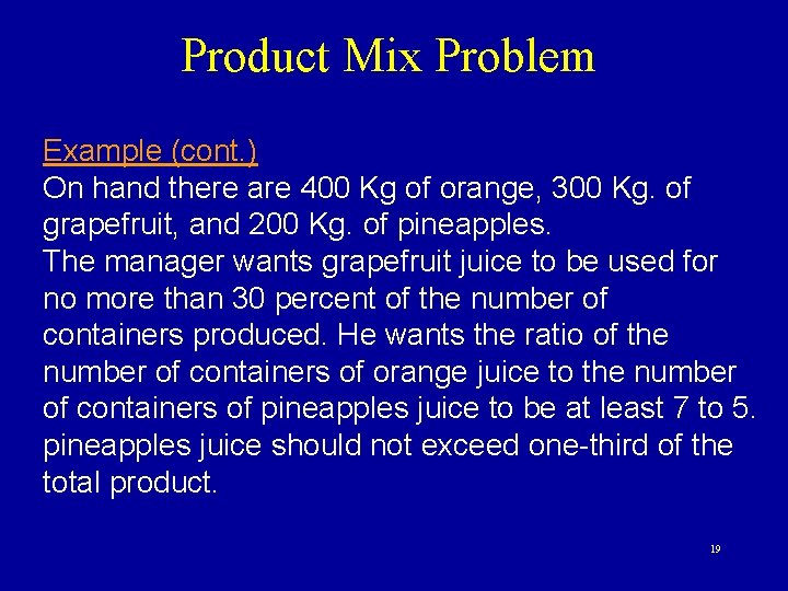
Product Mix Problem Example (cont. ) On hand there are 400 Kg of orange, 300 Kg. of grapefruit, and 200 Kg. of pineapples. The manager wants grapefruit juice to be used for no more than 30 percent of the number of containers produced. He wants the ratio of the number of containers of orange juice to the number of containers of pineapples juice to be at least 7 to 5. pineapples juice should not exceed one-third of the total product. 19

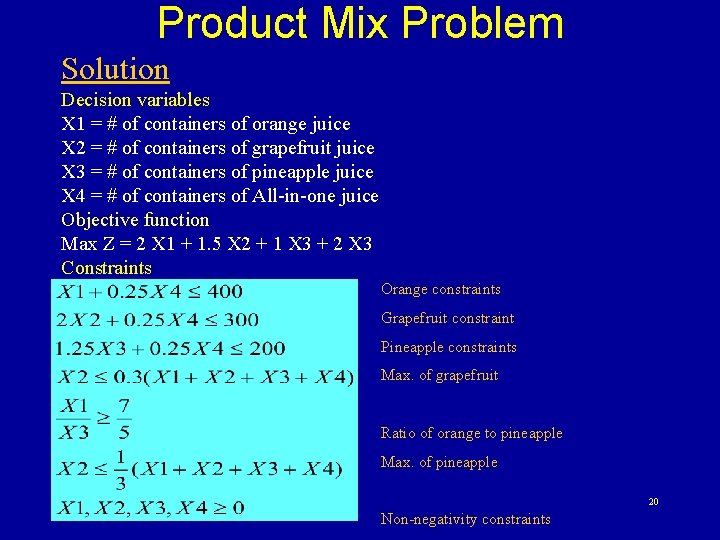
Product Mix Problem Solution Decision variables X 1 = # of containers of orange juice X 2 = # of containers of grapefruit juice X 3 = # of containers of pineapple juice X 4 = # of containers of All-in-one juice Objective function Max Z = 2 X 1 + 1. 5 X 2 + 1 X 3 + 2 X 3 Constraints Orange constraints Grapefruit constraint Pineapple constraints Max. of grapefruit Ratio of orange to pineapple Max. of pineapple 20 Non-negativity constraints

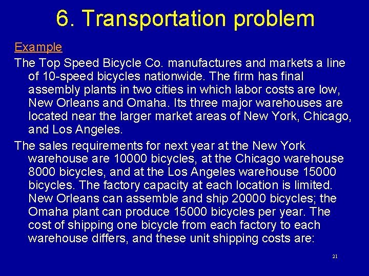
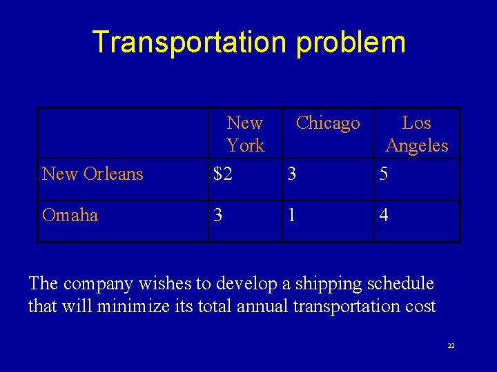
6. Transportation problem Example The Top Speed Bicycle Co. manufactures and markets a line of 10 -speed bicycles nationwide. The firm has final assembly plants in two cities in which labor costs are low, New Orleans and Omaha. Its three major warehouses are located near the larger market areas of New York, Chicago, and Los Angeles. The sales requirements for next year at the New York warehouse are 10000 bicycles, at the Chicago warehouse 8000 bicycles, and at the Los Angeles warehouse 15000 bicycles. The factory capacity at each location is limited. New Orleans can assemble and ship 20000 bicycles; the Omaha plant can produce 15000 bicycles per year. The cost of shipping one bicycle from each factory to each warehouse differs, and these unit shipping costs are: 21

Transportation problem New Orleans New York $2 Chicago 3 Los Angeles 5 Omaha 3 1 4 The company wishes to develop a shipping schedule that will minimize its total annual transportation cost 22

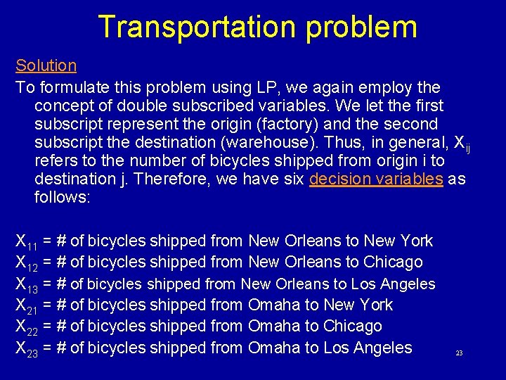
Transportation problem Solution To formulate this problem using LP, we again employ the concept of double subscribed variables. We let the first subscript represent the origin (factory) and the second subscript the destination (warehouse). Thus, in general, Xij refers to the number of bicycles shipped from origin i to destination j. Therefore, we have six decision variables as follows: X 11 = # of bicycles shipped from New Orleans to New York X 12 = # of bicycles shipped from New Orleans to Chicago X 13 = # of bicycles shipped from New Orleans to Los Angeles X 21 = # of bicycles shipped from Omaha to New York X 22 = # of bicycles shipped from Omaha to Chicago X 23 = # of bicycles shipped from Omaha to Los Angeles 23

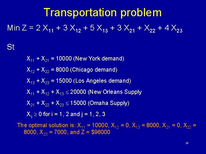
Transportation problem Min Z = 2 X 11 + 3 X 12 + 5 X 13 + 3 X 21 + X 22 + 4 X 23 St X 11 + X 21 = 10000 (New York demand) X 12 + X 22 = 8000 (Chicago demand) X 13 + X 23 = 15000 (Los Angeles demand) X 11 + X 12 + X 13 20000 (New Orleans Supply X 21 + X 22 + X 23 15000 (Omaha Supply) Xij 0 for i = 1, 2 and j = 1, 2, 3 The optimal solution is: X 11 = 10000, X 12 = 0, X 13 = 8000, X 21 = 0, X 22 = 8000, X 23 = 7000, and Z = $96000 24

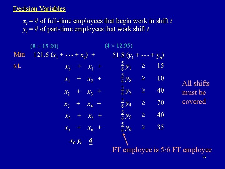
Decision Variables xt = # of full-time employees that begin work in shift t yt = # of part-time employees that work shift t (4 12. 95) (8 15. 20) Min s. t. 121. 6 (x 1 + • • • + x 6) + x 6 + x 1 + x 2 + x 3 + x 4 + x 5 + x 6 + xt, yt 0 51. 8 (y 1 + • • • + y 6) 5 6 5 6 5 6 y 1 15 y 2 10 y 3 40 y 4 70 y 5 40 y 6 35 All shifts must be covered PT employee is 5/6 FT employee 25

Terminology for solution of LP • A feasible solution is a solution for which all the constraints are satisfied. • A corner point feasible solution (CPF) is a feasible solution that lies at a corner point. • An infeasible solution is a solution for which at least one constraint is violated. • The feasible region is the collection of all feasible solution. • An Optimal solution is a feasible solution that has the most favorable value of the objective function. (it is always one of the CPF solution • The most favorable value is the largest (smallest) value if the objective function is to be maximized (minimized). 26

Graphical solution A Graphical Solution Procedure (LPs with 2 decision variables can be solved/viewed this way. ) 1. Plot each constraint as an equation and then decide which side of the line is feasible (if it’s an inequality). 2. Find the feasible region. 3. find the coordinates of the corner (extreme) points of the feasible region. 4. Substitute the corner point coordinates in the objective function 5. Choose the optimal solution 27

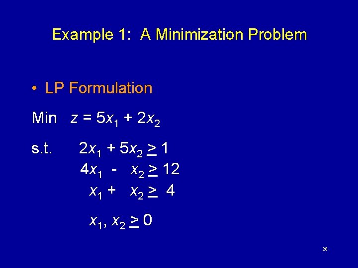
Example 1: A Minimization Problem • LP Formulation Min z = 5 x 1 + 2 x 2 s. t. 2 x 1 + 5 x 2 > 1 4 x 1 - x 2 > 12 x 1 + x 2 > 4 x 1, x 2 > 0 28

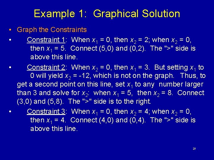
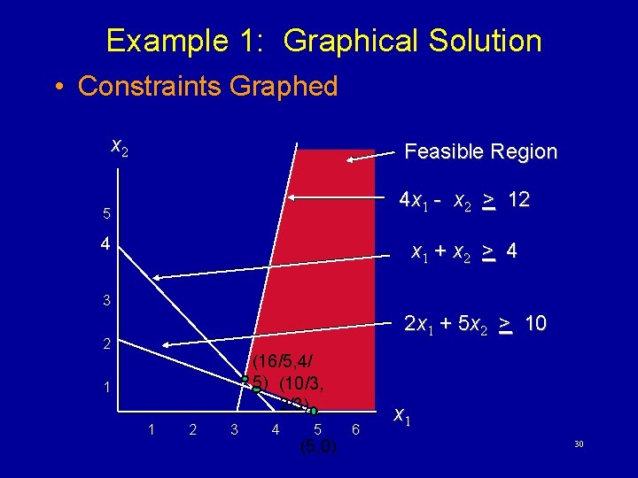
Example 1: Graphical Solution • Graph the Constraints • Constraint 1: When x 1 = 0, then x 2 = 2; when x 2 = 0, then x 1 = 5. Connect (5, 0) and (0, 2). The ">" side is above this line. • Constraint 2: When x 2 = 0, then x 1 = 3. But setting x 1 to 0 will yield x 2 = -12, which is not on the graph. Thus, to get a second point on this line, set x 1 to any number larger than 3 and solve for x 2: when x 1 = 5, then x 2 = 8. Connect (3, 0) and (5, 8). The ">" side is to the right. • Constraint 3: When x 1 = 0, then x 2 = 4; when x 2 = 0, then x 1 = 4. Connect (4, 0) and (0, 4). The ">" side is above this line. 29

Example 1: Graphical Solution • Constraints Graphed x 2 Feasible Region 4 x 1 - x 2 > 12 5 4 x 1 + x 2 > 4 3 2 x 1 + 5 x 2 > 10 2 (16/5, 4/ 5) (10/3, 2/3) 1 1 2 3 4 5 (5, 0) 6 x 1 30

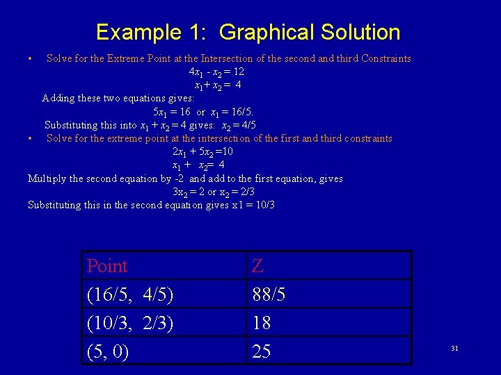
Example 1: Graphical Solution • Solve for the Extreme Point at the Intersection of the second and third Constraints 4 x 1 - x 2 = 12 x 1+ x 2 = 4 Adding these two equations gives: 5 x 1 = 16 or x 1 = 16/5. Substituting this into x 1 + x 2 = 4 gives: x 2 = 4/5 • Solve for the extreme point at the intersection of the first and third constraints 2 x 1 + 5 x 2 =10 x 1 + x 2= 4 Multiply the second equation by -2 and add to the first equation, gives 3 x 2 = 2 or x 2 = 2/3 Substituting this in the second equation gives x 1 = 10/3 Point (16/5, 4/5) (10/3, 2/3) (5, 0) Z 88/5 18 25 31

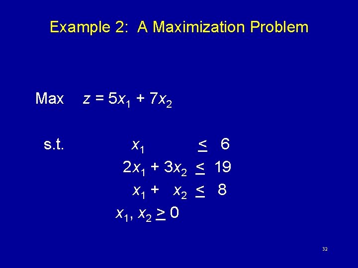
Example 2: A Maximization Problem Max s. t. z = 5 x 1 + 7 x 2 x 1 < 6 2 x 1 + 3 x 2 < 19 x 1 + x 2 < 8 x 1, x 2 > 0 32

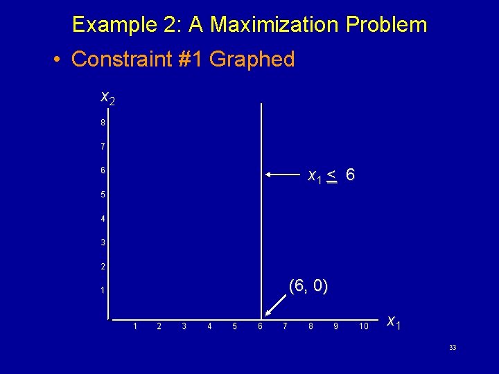
Example 2: A Maximization Problem • Constraint #1 Graphed x 2 8 7 x 1 < 6 6 5 4 3 2 (6, 0) 1 1 2 3 4 5 6 7 8 9 10 x 1 33

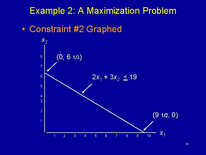
Example 2: A Maximization Problem • Constraint #2 Graphed x 2 (0, 6 1/3) 8 7 2 x 1 + 3 x 2 < 19 6 5 4 3 2 (9 1/2, 0) 1 1 2 3 4 5 6 7 8 9 10 x 1 34

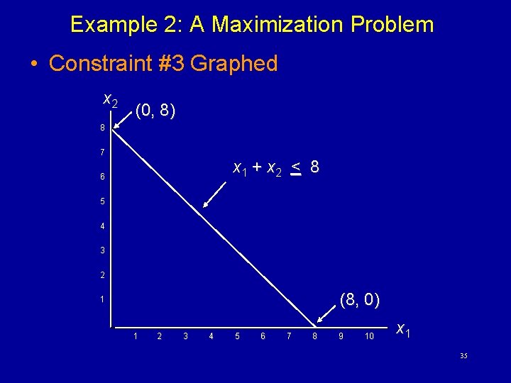
Example 2: A Maximization Problem • Constraint #3 Graphed x 2 (0, 8) 8 7 x 1 + x 2 < 8 6 5 4 3 2 (8, 0) 1 1 2 3 4 5 6 7 8 9 10 x 1 35

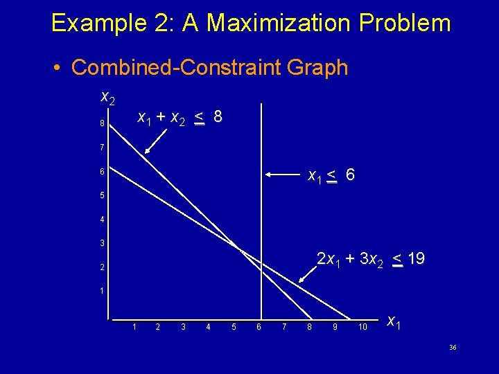
Example 2: A Maximization Problem • Combined-Constraint Graph x 2 8 x 1 + x 2 < 8 7 x 1 < 6 6 5 4 3 2 x 1 + 3 x 2 < 19 2 1 1 2 3 4 5 6 7 8 9 10 x 1 36

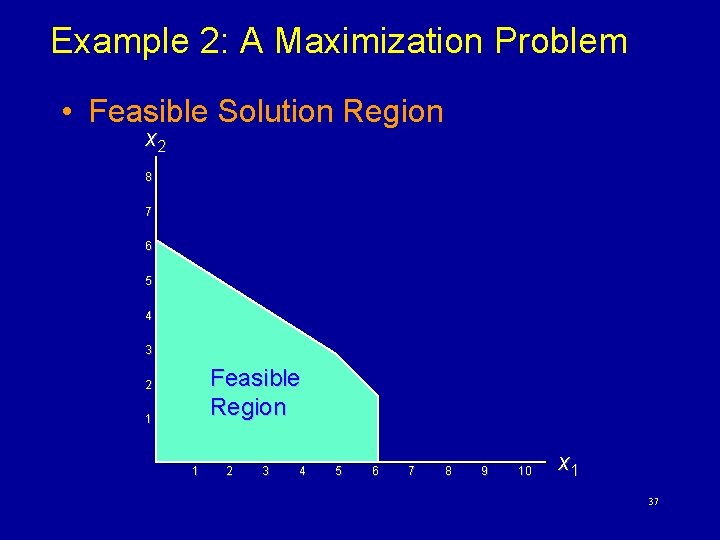
Example 2: A Maximization Problem • Feasible Solution Region x 2 8 7 6 5 4 3 Feasible Region 2 1 1 2 3 4 5 6 7 8 9 10 x 1 37

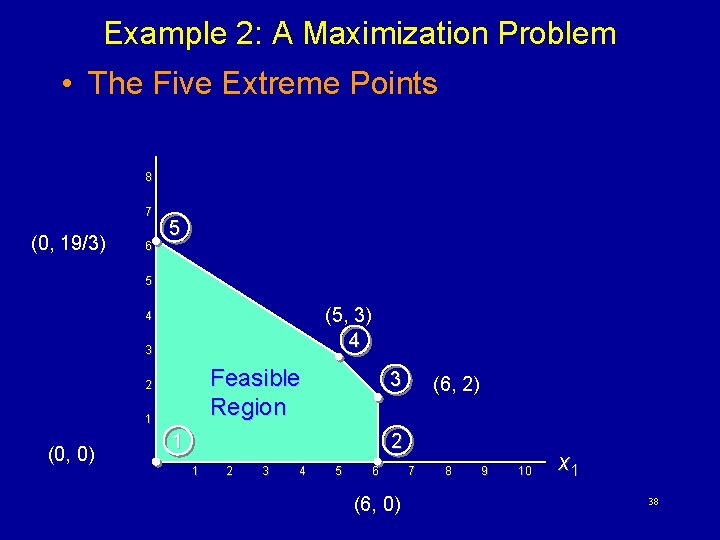
Example 2: A Maximization Problem • The Five Extreme Points 8 7 (0, 19/3) 6 5 5 (5, 3) 4 4 3 Feasible Region 2 1 (0, 0) 3 1 (6, 2) 2 1 2 3 4 5 6 (6, 0) 7 8 9 10 x 1 38

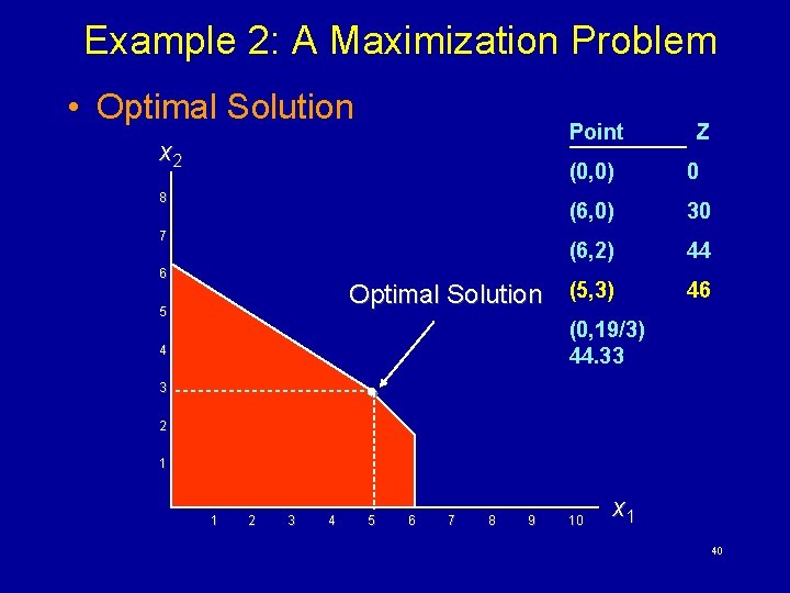
Example 2: A Maximization Problem • Having identified the feasible region for the problem, we now search for the optimal solution, which will be the point in the feasible region with the largest (in case of maximization or the smallest (in case of minimization) of the objective function. • To find this optimal solution, we need to evaluate the objective function at each one of the corner points of the feasible region. 39

Example 2: A Maximization Problem • Optimal Solution Point x 2 (0, 0) 0 (6, 0) 30 (6, 2) 44 Optimal Solution (5, 3) 46 8 7 6 5 Z (0, 19/3) 44. 33 4 3 2 1 1 2 3 4 5 6 7 8 9 10 x 1 40

Extreme Points and the Optimal Solution • The corners or vertices of the feasible region are referred to as the extreme points. • An optimal solution to an LP problem can be found at an extreme point of the feasible region. • When looking for the optimal solution, you do not have to evaluate all feasible solution points. • You have to consider only the extreme points of the feasible region. 41

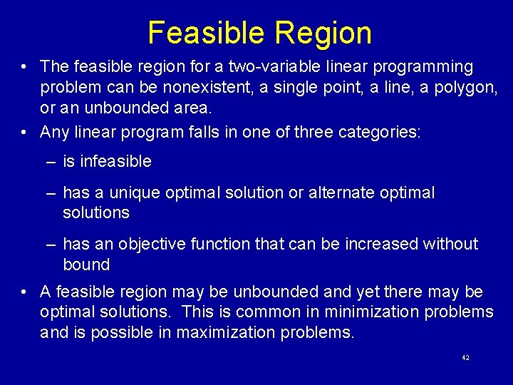
Feasible Region • The feasible region for a two-variable linear programming problem can be nonexistent, a single point, a line, a polygon, or an unbounded area. • Any linear program falls in one of three categories: – is infeasible – has a unique optimal solution or alternate optimal solutions – has an objective function that can be increased without bound • A feasible region may be unbounded and yet there may be optimal solutions. This is common in minimization problems and is possible in maximization problems. 42

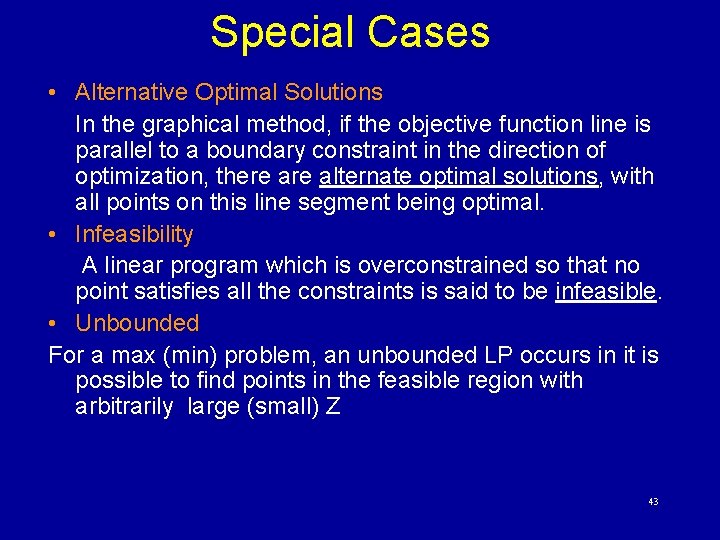
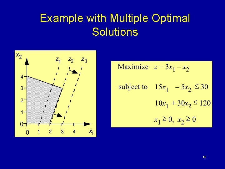
Special Cases • Alternative Optimal Solutions In the graphical method, if the objective function line is parallel to a boundary constraint in the direction of optimization, there alternate optimal solutions, with all points on this line segment being optimal. • Infeasibility A linear program which is overconstrained so that no point satisfies all the constraints is said to be infeasible. • Unbounded For a max (min) problem, an unbounded LP occurs in it is possible to find points in the feasible region with arbitrarily large (small) Z 43

Example with Multiple Optimal Solutions 44

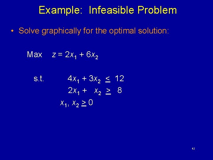
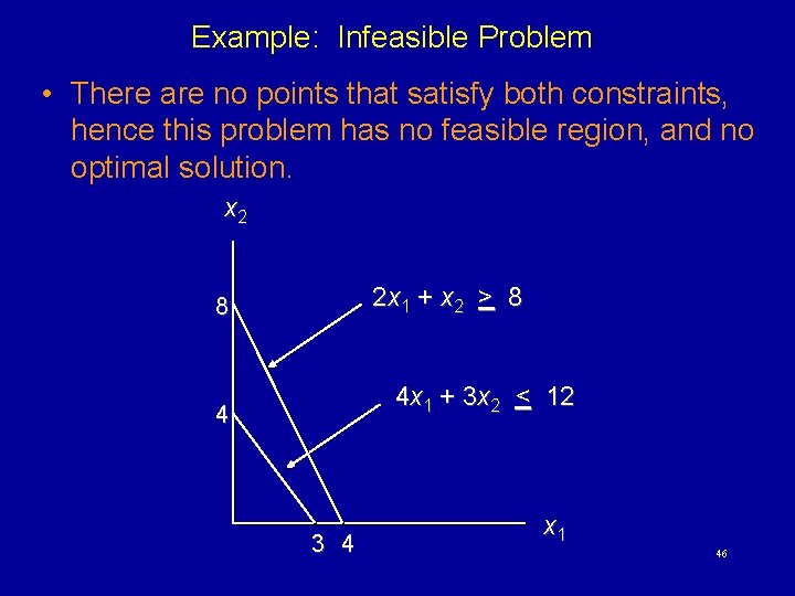
Example: Infeasible Problem • Solve graphically for the optimal solution: Max s. t. z = 2 x 1 + 6 x 2 4 x 1 + 3 x 2 < 12 2 x 1 + x 2 > 8 x 1, x 2 > 0 45

Example: Infeasible Problem • There are no points that satisfy both constraints, hence this problem has no feasible region, and no optimal solution. x 2 2 x 1 + x 2 > 8 8 4 x 1 + 3 x 2 < 12 4 3 4 x 1 46

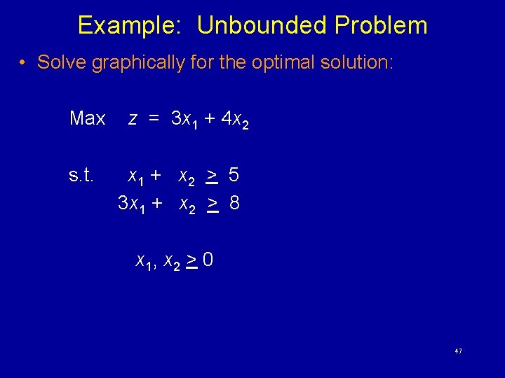
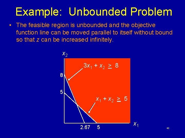
Example: Unbounded Problem • Solve graphically for the optimal solution: Max s. t. z = 3 x 1 + 4 x 2 x 1 + x 2 > 5 3 x 1 + x 2 > 8 x 1, x 2 > 0 47

Example: Unbounded Problem • The feasible region is unbounded and the objective function line can be moved parallel to itself without bound so that z can be increased infinitely. x 2 3 x 1 + x 2 > 8 8 5 x 1 + x 2 > 5 2. 67 5 x 1 48

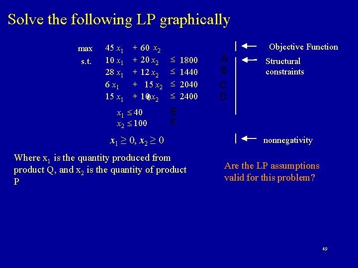
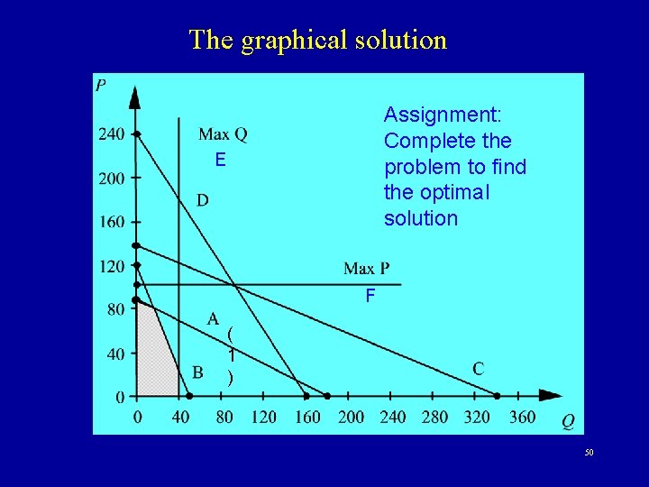
Solve the following LP graphically max s. t. 45 x 1 10 x 1 28 x 1 6 x 1 15 x 1 + + + 60 x 2 20 x 2 12 x 2 15 x 2 100 x 2 x 1 40 x 2 100 Objective Function 1800 1440 2040 2400 A B C D Structural constraints E F x 1 ≥ 0, x 2 ≥ 0 Where x 1 is the quantity produced from product Q, and x 2 is the quantity of product P nonnegativity Are the LP assumptions valid for this problem? 49

The graphical solution Assignment: Complete the problem to find the optimal solution E F ( 1 ) 50

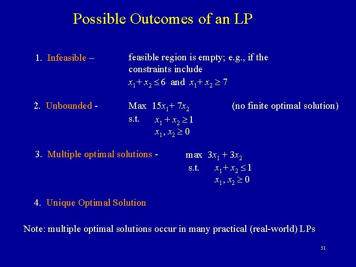
Possible Outcomes of an LP 1. Infeasible – feasible region is empty; e. g. , if the constraints include x 1+ x 2 6 and x 1+ x 2 7 2. Unbounded - Max 15 x 1+ 7 x 2 s. t. x 1 + x 2 1 x 1 , x 2 0 3. Multiple optimal solutions - (no finite optimal solution) max 3 x 1 + 3 x 2 s. t. x 1 + x 2 1 x 1 , x 2 0 4. Unique Optimal Solution Note: multiple optimal solutions occur in many practical (real-world) LPs. 51