CHAPTER 2 Key Concepts of Urban Economics Mc
CHAPTER 2 Key Concepts of Urban Economics ©Mc. Graw-Hill Education. All rights reserved. Authorized only for instructor use in the classroom. No reproduction or further distribution permitted without the prior written consent of Mc. Graw-Hill Education.

Six Key Concepts from Microeconomics Six key concepts from microeconomics provide a foundation for urban economics: 1. Opportunity Cost 2. Marginal Principle 3. Nash Equilibrium 4. Comparative Statics 5. Pareto Efficiency 6. Self-Reinforcing Changes ©Mc. Graw-Hill Education.
1. Opportunity Cost Economic cost is opportunity cost. • The opportunity cost is what you sacrifice to get something. • The opportunity cost of a resource is its value in its next-best use. • Economic cost can be divided into two types: – Explicit cost that involves an explicit monetary payment for an input. – Implicit cost is the opportunity cost of inputs that are not subject to an explicit monetary payment. There are two types of implicit cost: • Opportunity cost of an entrepreneur’s time. • Opportunity cost of an entrepreneur’s funds ©Mc. Graw-Hill Education.
1. Opportunity Cost (cont. ) In the example of building a skyscraper: • What would be the opportunity cost of the entrepreneur’s funds? • What would be the opportunity cost of the entrepreneur’s time? ` ©Mc. Graw-Hill Education.
1. Opportunity Cost (cont. ) • Examples: urban environment – opportunity cost of travel time is value of time in next best use – opportunity cost of housing is value of capital as factory or school – opportunity cost of open space is value of developed land – opportunity cost of a light-rail system is bus fleet – opportunity cost of prison time is foregone production – opportunity cost of prison facility is value of capital in other use ©Mc. Graw-Hill Education.
2. Marginal Principle: Choose the level of an activity at which the marginal benefit equals the marginal cost. • Marginal benefit: additional benefit from one more unit • Marginal cost: additional cost requited to provide the benefit of one more unit ©Mc. Graw-Hill Education.
The Marginal Principle (cont. ) ©Mc. Graw-Hill Education.
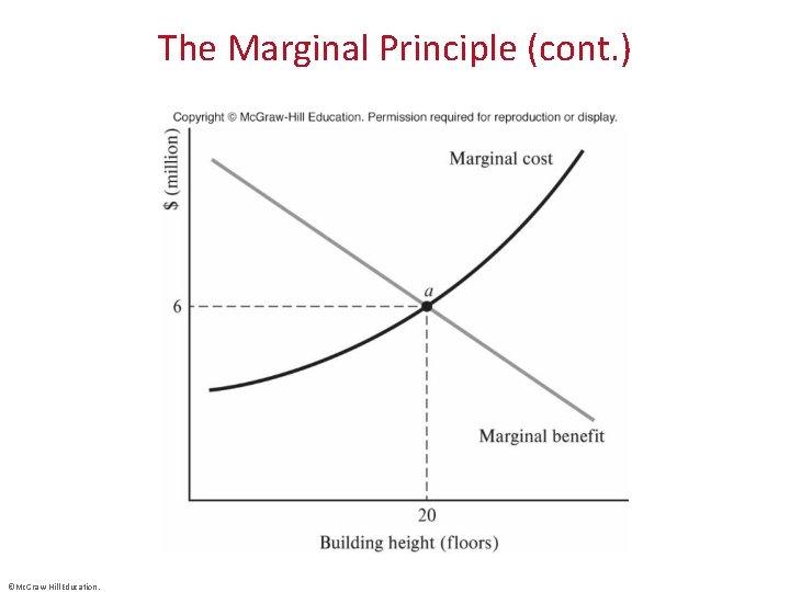
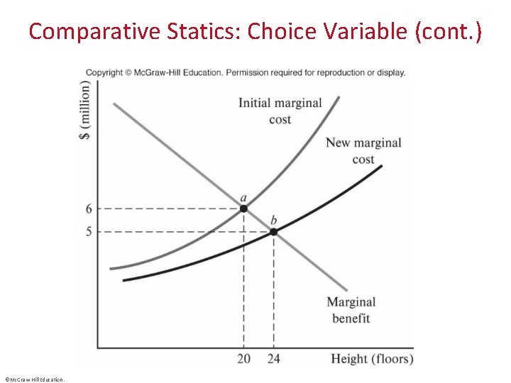
The Marginal Principle (cont. ) 1. Marginal benefit: The marginal benefit of the building height equals the rent collected on the additional floor. The marginal-benefit curve is negatively sloped, because a taller building devotes more space to vertical transportation (stairs and elevators), leaving less rentable space. As the number of floors increases, total rental revenue increases, but at a decreasing rate. 2. Marginal cost: The marginal cost of the building height equals the additional construction cost from building one more floor. The marginal-cost curve is positively sloped because a taller building requires more reinforcement to support its more concentrated weight. As the number of floors increases, construction cost increases at an increasing rate. The firm maximizes profit at point a, with 20 floors at a marginal cost of $6 million. The firm stops at 20 floors because the cost of adding the 21 st floor exceeds the rental revenue from the additional floor. ©Mc. Graw-Hill Education.
2. Marginal Principle (cont. ) Urban applications: • Households use the marginal principle in choosing a residential location and how to vote in local elections. • Firms use the marginal principle to decide how much to produce, how many workers to hire, and where to locate a production facility. • Local governments use the marginal principle to make decisions on hiring teachers, public-safety programs, buses. ©Mc. Graw-Hill Education.
3. Nash Equilibrium: There is no incentive for unilateral deviation. • Nash equilibrium is achieved if the following occurs. – No single decision-maker has an incentive to change his or her behavior, given the choices made by other participants. – There are no regrets, given the choices of other participants. ©Mc. Graw-Hill Education.
Nash Equilibrium in a Supply and Demand Model Key assumptions of the Supply and Demand Model: • Both consumers and producers in a perfectly competitive market are price takers. – Firms cannot unilaterally move the price in a favorable direction. – Consumers cannot move the price in a favorable direction. ©Mc. Graw-Hill Education.
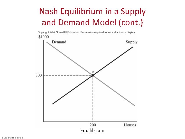
Nash Equilibrium in a Supply and Demand Model (cont. ) Equilibrium ©Mc. Graw-Hill Education.
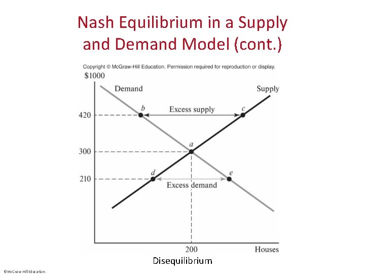
Nash Equilibrium in a Supply and Demand Model (cont. ) Disequilibrium ©Mc. Graw-Hill Education.
Nash Equilibrium in Location Choice The concept of Nash equilibrium applies to all sorts of decisionmaking environments. • Example: vendors compete for customers on a beach – Two vendors sell vanilla ice cream along a beach that is 11 blocks long. – Consumers are uniformly distributed along the beach, with one customer on each block. – Each consumer patronizes the closest ice-cream vendor. ©Mc. Graw-Hill Education.
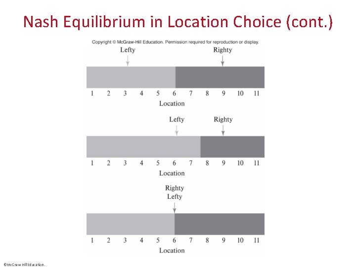
Nash Equilibrium in Location Choice (cont. ) ©Mc. Graw-Hill Education.
Nash Equilibrium in Location Choice In the initial location pattern shown in the previous slide, vendors Lefty and Righty divide the beach into two equal market areas, and each locates at the center of his or her market. Lefty’s consumers are in blocks 1 through 5, while Righty’s customers are in blocks 7 through 11. The consumer in block 6 is indifferent and choose a vendor randomly. Each vendor has five customers for certain and a 50 -50 chance at a sixth customer. Although the initial location pattern seems sensible, it is not a Nash equilibrium because each vendor has an incentive to unilaterally deviate. The second and third panels show the transition from the initial positions (in the upper panel) to the Nash equilibrium. Let’s talk about the second/middle panel. Here, Lefty moves to the median location. Suppose Lefty moves to block 6. This is the median location, defined as the location that splits consumers into two equal groups: five consumers are to the left, and five customers are to the right. Lefty’s unilateral deviation increases her number of customers to seven. In contrast, Righty now has only four consumers. ©Mc. Graw-Hill Education.
Nash Equilibrium and Spatial Variation in Prices • Location – Higher price for a more desirable location eliminates the incentive for unilateral deviation (move to more desirable location). • Labor markets – Lower wage for a more desirable workplace eliminates the incentive for unilateral deviation (move to more desirable workplace). ©Mc. Graw-Hill Education.
4. Comparative Statics Comparative statics are used to predict the responses of decisionmakers and markets to changes in economic circumstances. • The two types of comparative-statics exercises are: – comparative statics for a choice variable – comparative statics for an equilibrium variable. ©Mc. Graw-Hill Education.
Comparative Statics: Choice Variable • Parameter – a variable whose value is taken as given by a decision-maker • Comparative statics – effect of change in the value of a parameter on the value of a choice variable • Example – increase in the price of steel (a parameter to the builder) decreases the profit-maximizing building height (the choice variable) ©Mc. Graw-Hill Education.
Comparative Statics: Choice Variable (cont. ) ©Mc. Graw-Hill Education. .
Comparative Statics: Choice Variable • The urban economy provides many opportunities to do comparative statics for choice variables. • Other urban comparative-statics exercises include – transport cost and firm location – transit service and transit ridership – change in neighbors and household location ©Mc. Graw-Hill Education.

Comparative Statics: Equilibrium Variable • Parameter – a variable whose value is determined outside the market being studied • Comparative statics – the effect of a change in the value of a parameter on the value of an equilibrium variable • Example – increase in price of fertilizer (parameter for apple market) increases equilibrium price of apples ©Mc. Graw-Hill Education.
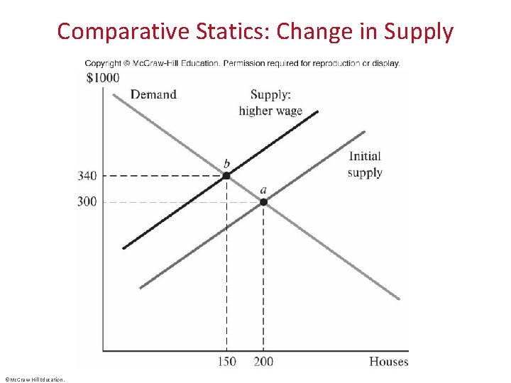
Comparative Statics: Change in Supply ©Mc. Graw-Hill Education. .
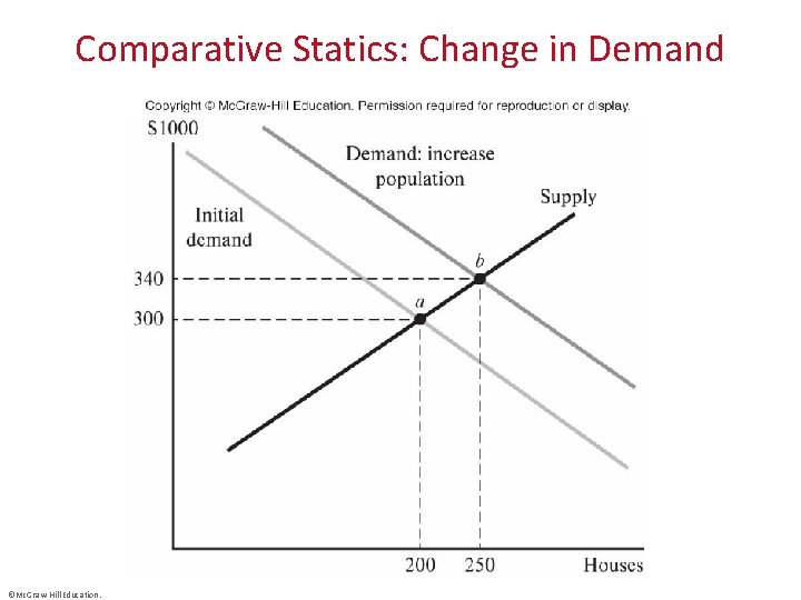
Comparative Statics: Change in Demand ©Mc. Graw-Hill Education. .
Comparative Statics: Equilibrium Variable • The urban economy provides many opportunities to do comparative statics for market equilibria. • Other urban comparative-statics exercises include: – labor demand wage – land policy and price of land – congestion tax and traffic volume ©Mc. Graw-Hill Education.
5. Pareto Efficiency Pareto efficiency is an economic state where resources are allocated in the most efficient manner. It is obtained when a distribution strategy exists where one party’s situation cannot be improved without making another party's situation worse. • Pareto improvement entails a reallocation of resources that makes at least one person better off without making anyone worse off. – An allocation is Pareto inefficient if there is a Pareto improvement. – An allocation is Pareto efficient there is no Pareto improvement. ©Mc. Graw-Hill Education.
Pareto Efficiency: Island Economy ©Mc. Graw-Hill Education. .
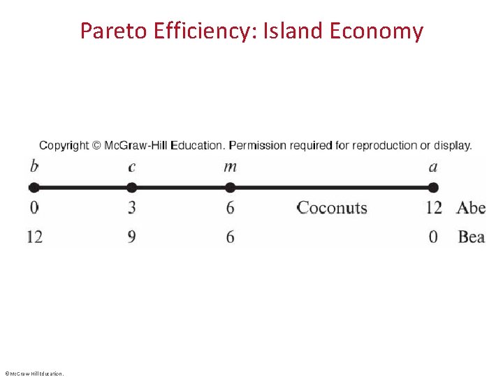
Pareto Efficiency: Island Economy In this example, an island economy has 12 coconuts to divide between two people, Abe and Bea. Every allocation of the coconuts between the two people is Pareto efficient because any reallocation of coconuts makes one person better off at the expense of the other. Starting at point b, we can make Abe better off by giving him his first coconut, but only by taking a coconut from Bea and making her worse off. Similarly, starting at point c, Abe could go from 3 to 4 coconuts, but only if Bea goes from 9 to 8 coconuts. Each allocation is Pareto efficient because any change harms someone. This simple example highlights the distinction between economic efficiency and equity or fairness. A 50 -50 split of the coconuts may be appealing for reasons of equity or fairness, but an equal division is one of many efficient allocations. In a real economy, there are many efficient allocations of resources and goods across consumers, and reasonable people can disagree about which efficient allocation is the most equitable. ©Mc. Graw-Hill Education. .

Market Equilibrium and Pareto Efficiency Market equilibrium is Pareto efficient when four conditions are satisfied: 1. Firms do not control prices but instead take the market price as given. 2. All the costs of production are incurred by firms. 3. No external party benefits in consumption and production 4. There is perfect information for consumers and producers. – Consumers are informed about product characteristics. – Producers are informed about cost of serving customers. ©Mc. Graw-Hill Education.
Pareto Inefficiency in the Urban Economy In an urban economy, the second efficiency condition—no external cost—is sometimes violated, generating Pareto inefficient allocations. • In the example of air pollution caused by one ton of sulphur dioxide: – Health costs of $500 could be avoided at an abatement cost of $100. – Pareto improvement could be achieved by splitting the difference to make both parties better off by $200. ©Mc. Graw-Hill Education.
Pareto Inefficiency in the Urban Economy (cont. ) In an urban economy, the second efficiency condition—no external cost—is sometimes violated, generating Pareto inefficient allocations. • In the example of congestion caused by a marginal driver slowing traffic on the high way: – External cost: congestion from marginal driver’s use of road • Each of 100 drivers bears additional time cost of $0. 07 • Value of trip = $2 • Drivers pay $3 ($0. 03) to keep marginal driver off road – External benefit: public goods and firm clustering ©Mc. Graw-Hill Education.

6. Self-Reinforcing Changes The typical market analysis in microeconomics involves markets subject to self-limiting changes in market conditions. • Case of self-limiting changes leading to non-extreme outcomes include: – increase in demand causes excess demand, increasing price – increase in price decreases excess demand as quantity demanded increases and quantity supplied increases – new equilibrium—quantity between initial and new (before ∆p) ©Mc. Graw-Hill Education.
Self-Reinforcing Changes: Auto Row ©Mc. Graw-Hill Education. .
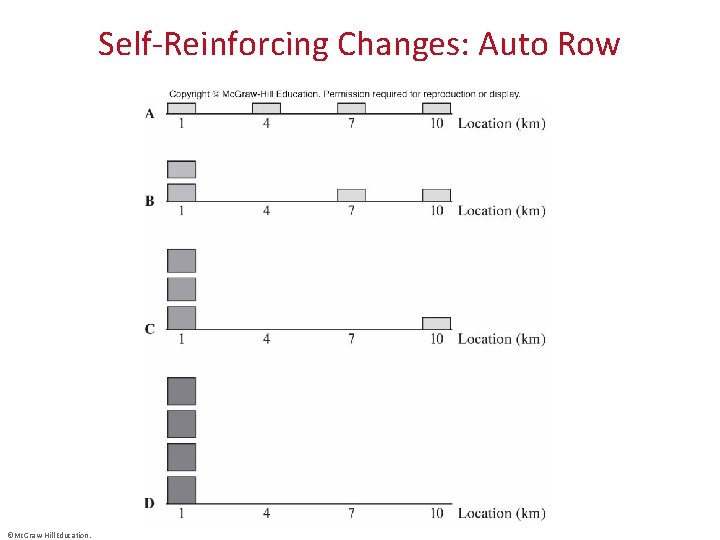
Self-Reinforcing Changes: Auto Row The previous slide illustrates the effects of self-reinforcing changes by considering the location of automobile sellers. Suppose four sellers are initially distributed uniformly throughout a city and earn the same profit. Panel A: We see small profit rectangles. If one seller moves to a location next to another seller, what happens next? Panel B: Auto consumers compare brands before buying. The two-firm cluster will facilitate comparison shopping, so the number of car shoppers at location 1 will more than double. The profit per firm increases, as indicated by the larger profit rectangles for firms in the cluster. Panel C: The higher profit in the cluster attracts a third firm, causing a disproportionate increase in the number of shoppers, a result of enhanced comparison shopping. The cluster profit increases, increasing the profit gap between a firm in the cluster and the isolated firm at location 10. Panel D: The fourth firm joins other firms in the cluster, causing a disproportionate increase in the number of shoppers and an increase in profit per firm. ©Mc. Graw-Hill Education. .
Self-Reinforcing Changes: Other Examples • Other examples of self-reinforcing effects in urban area include – clustering of artists to promote exposure and decrease costs – clustering of consumers to consume products with low per-capita demand – clustering of like-minded people (residential segregation) ©Mc. Graw-Hill Education.
- Slides: 35