Chapter 2 Introduction to Linear Programming Learning Objectives

Chapter 2 Introduction to Linear Programming

Learning Objectives • • • Formulate a maximization problem Use graphical solution procedure Identify feasible solution space Define extreme points and optimal solution Formulate a minimization problem. Set up standard form of an LP problem

Introduction • Many decisions focus on the best way to achieve the objectives of business subject to the restrictions • Restrictions take the form of limited resources • One objective of firms is to maximize profit or to minimize cost • Linear Programming is to optimize the usage of limited resources • Derives its name from the functional relationships that are linear and the solution consists of mathematical steps, that is, a program

Construction of LP Model • Formulation of model that represents the problem, and then solve it • Three steps in applying LP technique • First, problem must be identified • Second, problem must be formulated • Third, model must be solved

Model Formulation • Consists of certain components • Components include decision variables, objective function, and constraints • Decision variables represent levels of activity • Objective function describes objective of firm – Consists of either maximizing or minimizing some value • Constraints are linear relationships of decision variable – Represent restrictions placed on firm

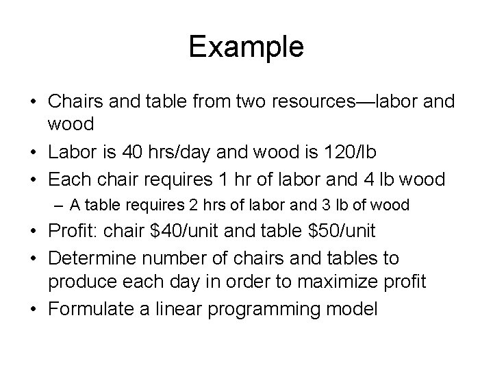
Example • Chairs and table from two resources—labor and wood • Labor is 40 hrs/day and wood is 120/lb • Each chair requires 1 hr of labor and 4 lb wood – A table requires 2 hrs of labor and 3 lb of wood • Profit: chair $40/unit and table $50/unit • Determine number of chairs and tables to produce each day in order to maximize profit • Formulate a linear programming model

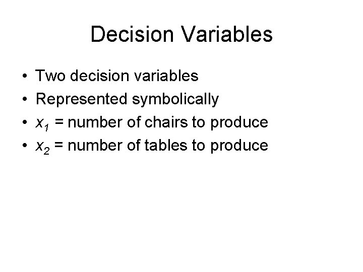
Decision Variables • • Two decision variables Represented symbolically x 1 = number of chairs to produce x 2 = number of tables to produce

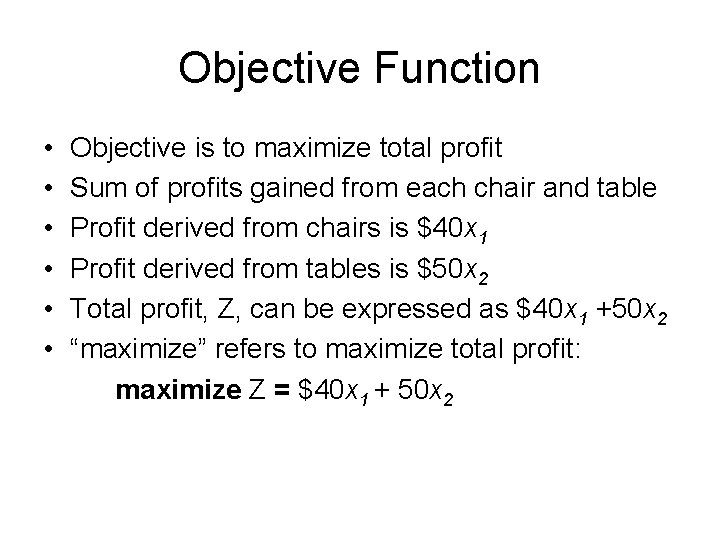
Objective Function • • • Objective is to maximize total profit Sum of profits gained from each chair and table Profit derived from chairs is $40 x 1 Profit derived from tables is $50 x 2 Total profit, Z, can be expressed as $40 x 1 +50 x 2 “maximize” refers to maximize total profit: maximize Z = $40 x 1 + 50 x 2

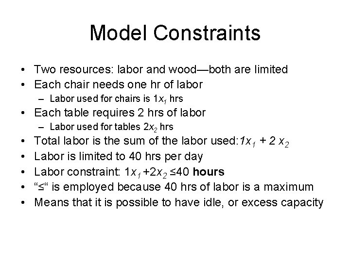
Model Constraints • Two resources: labor and wood—both are limited • Each chair needs one hr of labor – Labor used for chairs is 1 x 1 hrs • Each table requires 2 hrs of labor – Labor used for tables 2 x 2 hrs • • • Total labor is the sum of the labor used: 1 x 1 + 2 x 2 Labor is limited to 40 hrs per day Labor constraint: 1 x 1 +2 x 2 ≤ 40 hours “≤“ is employed because 40 hrs of labor is a maximum Means that it is possible to have idle, or excess capacity

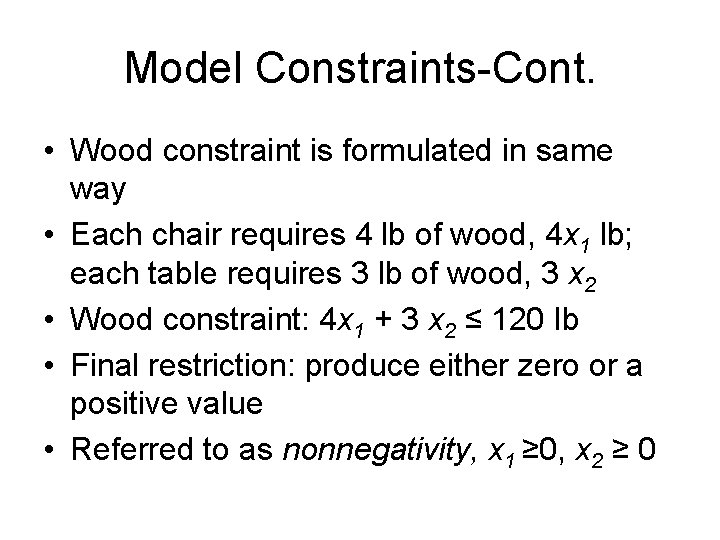
Model Constraints-Cont. • Wood constraint is formulated in same way • Each chair requires 4 lb of wood, 4 x 1 lb; each table requires 3 lb of wood, 3 x 2 • Wood constraint: 4 x 1 + 3 x 2 ≤ 120 Ib • Final restriction: produce either zero or a positive value • Referred to as nonnegativity, x 1 ≥ 0, x 2 ≥ 0

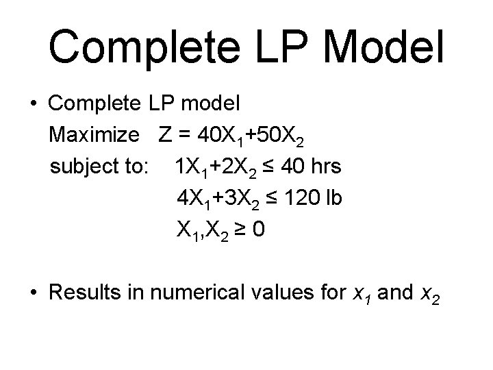
Complete LP Model • Complete LP model Maximize Z = 40 X 1+50 X 2 subject to: 1 X 1+2 X 2 ≤ 40 hrs 4 X 1+3 X 2 ≤ 120 lb X 1, X 2 ≥ 0 • Results in numerical values for x 1 and x 2

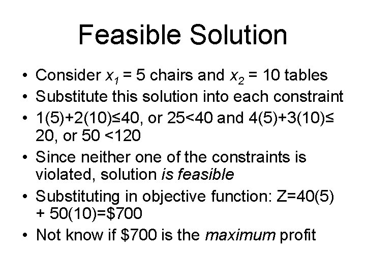
Feasible Solution • Consider x 1 = 5 chairs and x 2 = 10 tables • Substitute this solution into each constraint • 1(5)+2(10)≤ 40, or 25<40 and 4(5)+3(10)≤ 20, or 50 <120 • Since neither one of the constraints is violated, solution is feasible • Substituting in objective function: Z=40(5) + 50(10)=$700 • Not know if $700 is the maximum profit

Infeasible Solution • • • x 1 =10 chairs and x 2 = 20 tables Results Z= $40(10)+50(20)=$1, 400 Infeasible: violates labor constraint Maximize Z without violating constraints Optimal solution can be found using graphical solution approach

Graphical Solution • Provides a picture of how a solution is obtained • Limited to only two decision variables • For three decision variables: cumbersome • Useful: gives a "picture" of how a solution is derived • Also provides how computer and mathematical solution approaches work

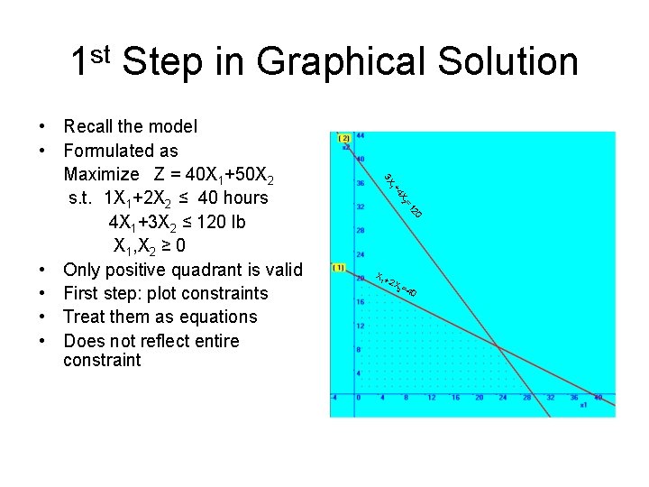
1 st Step in Graphical Solution 20 =1 X 2 +4 1 3 X • Recall the model • Formulated as Maximize Z = 40 X 1+50 X 2 s. t. 1 X 1+2 X 2 ≤ 40 hours 4 X 1+3 X 2 ≤ 120 lb X 1, X 2 ≥ 0 • Only positive quadrant is valid • First step: plot constraints • Treat them as equations • Does not reflect entire constraint X+ 1 2 X= 2 4 0

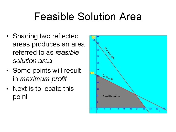
Feasible Solution Area 20 =1 X 2 +4 1 3 X • Shading two reflected areas produces an area referred to as feasible solution area • Some points will result in maximum profit • Next is to locate this point X+ 1 2 X= 2 4 0 Feasible region

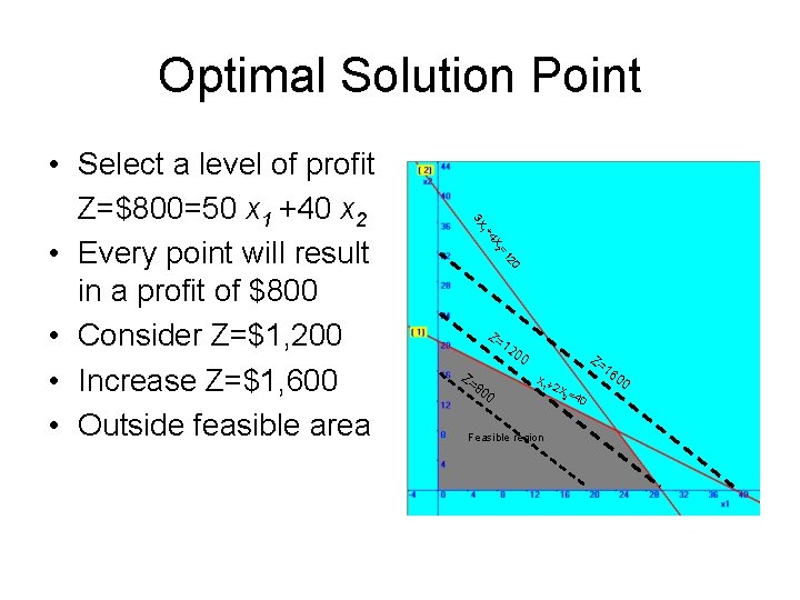
Optimal Solution Point 20 =1 X 2 +4 1 3 X • Select a level of profit Z=$800=50 x 1 +40 x 2 • Every point will result in a profit of $800 • Consider Z=$1, 200 • Increase Z=$1, 600 • Outside feasible area Z= 12 0 0 Z= 80 0 Z= X+ 1 2 X= 2 4 0 Feasible region 16 00

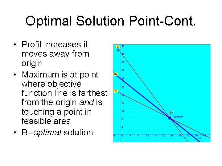
Optimal Solution Point-Cont. • Profit increases it moves away from origin • Maximum is at point where objective function line is farthest from the origin and is touching a point in feasible area • B--optimal solution B

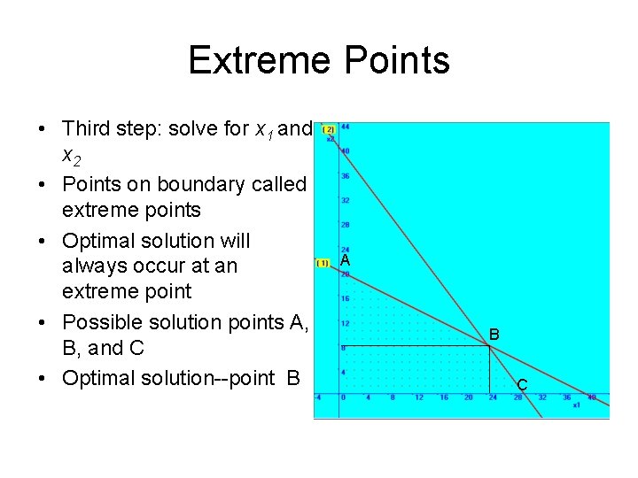
Extreme Points • Third step: solve for x 1 and x 2 • Points on boundary called extreme points • Optimal solution will always occur at an extreme point • Possible solution points A, B, and C • Optimal solution--point B A B C

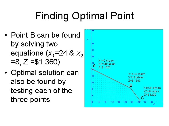
Finding Optimal Point • Point B can be found by solving two equations (x 1=24 & x 2 =8, Z =$1, 360) • Optimal solution can also be found by testing each of the three points A X 1=0 chairs X 2=20 tables Z=$ 1000 X 1=24 chairs X 2=8 tables Z=$ 1360 B C X 1=30 chairs X 2=0 tables Z=$ 1200

Graphical Solution Steps • Steps are as follows 1. Plot all model constraints as equations 2. Indicate feasible solution area 3. Determine corner points; then, find the solution values at each point 4. Substitute these values into objective function

Minimization Problem • Two LP problems, a maximization and a minimization • Minimization is formulated in the same way, except for a few minor differences • Show to formulate a minimization problem

A Minimization Problem • Razi makes fertilizer from two ingredients • Ingredients A and B provide different amounts of potassium and nitrogen • A provides 2 ounces of potassium and 4 ounces of nitrogen, whereas ingredient B provides 3 ounces of nitrogen and 4 ounces of potassium • A and B cost $6 and $3 per pound • How many pounds of each ingredient to put into a bag of fertilizer to meet minimum requirements of 16 ounces of potassium and 24 ounces of nitrogen while minimizing cost • Formulate a LP model

Decision Variables and Objective Function • Two decision variables representing the number of lbs of each ingredient x 1=lb of ingredient 1 x 2=lb of ingredient 2 • Objective: minimize total purchase cost of ingredients • Expressed Min Z = 6 x 1 + 3 x 2

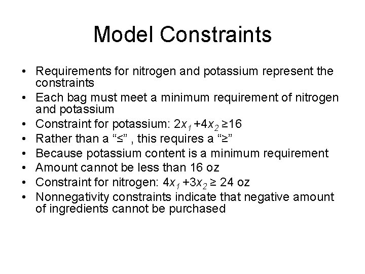
Model Constraints • Requirements for nitrogen and potassium represent the constraints • Each bag must meet a minimum requirement of nitrogen and potassium • Constraint for potassium: 2 x 1 +4 x 2 ≥ 16 • Rather than a “≤” , this requires a “≥” • Because potassium content is a minimum requirement • Amount cannot be less than 16 oz • Constraint for nitrogen: 4 x 1 +3 x 2 ≥ 24 oz • Nonnegativity constraints indicate that negative amount of ingredients cannot be purchased

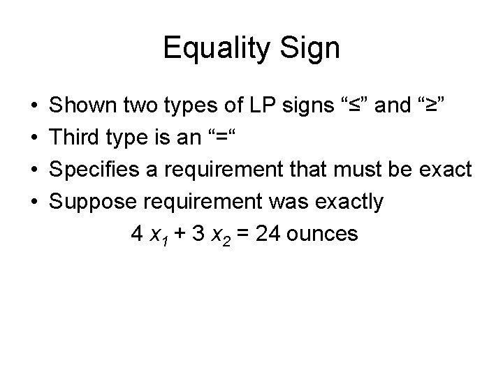
Equality Sign • • Shown two types of LP signs “≤” and “≥” Third type is an “=“ Specifies a requirement that must be exact Suppose requirement was exactly 4 x 1 + 3 x 2 = 24 ounces

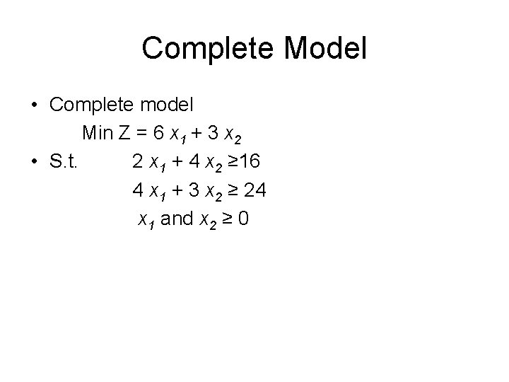
Complete Model • Complete model Min Z = 6 x 1 + 3 x 2 • S. t. 2 x 1 + 4 x 2 ≥ 16 4 x 1 + 3 x 2 ≥ 24 x 1 and x 2 ≥ 0

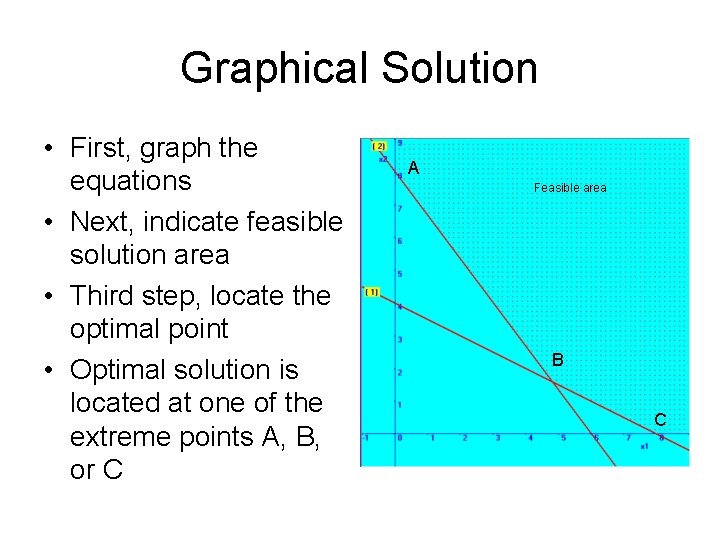
Graphical Solution • First, graph the equations • Next, indicate feasible solution area • Third step, locate the optimal point • Optimal solution is located at one of the extreme points A, B, or C A Feasible area B C

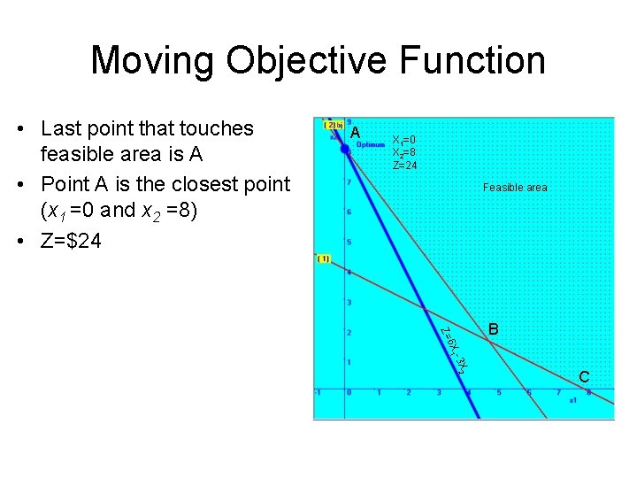
Moving Objective Function • Last point that touches feasible area is A • Point A is the closest point (x 1 =0 and x 2 =8) • Z=$24 A X 1=0 X 2=8 Z=24 Feasible area -3 X 2 6 X 1 Z= B C

Limitation of Graphical Solution • Learned how a LP model is formulated and how a solution can be derived • Graphing provides valuable insight into LP • Limited to only two decision variables • Will show LP problems can be solved using computer software packages

Slack Variable • • Graphical does not provide all the information Need to transform the model into standard form Necessary for interpretation of LP solutions Recall the maximization example Solution occurred at an extreme point Constraints must all be in the form of equations “=“ Procedure for transforming “≤” constraints into “=“ Achieved by adding a new variable, called a slack variable

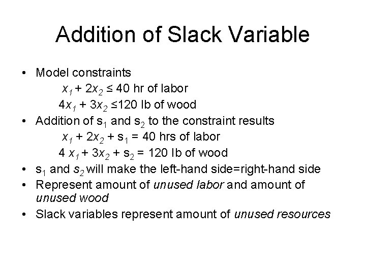
Addition of Slack Variable • Model constraints x 1 + 2 x 2 ≤ 40 hr of labor 4 x 1 + 3 x 2 ≤ 120 lb of wood • Addition of s 1 and s 2 to the constraint results x 1 + 2 x 2 + s 1 = 40 hrs of labor 4 x 1 + 3 x 2 + s 2 = 120 Ib of wood • s 1 and s 2 will make the left-hand side=right-hand side • Represent amount of unused labor and amount of unused wood • Slack variables represent amount of unused resources

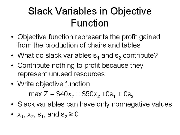
Slack Variables in Objective Function • Objective function represents the profit gained from the production of chairs and tables • What do slack variables s 1 and s 2 contribute? • Contribute nothing to profit because they represent unused resources • Write objective function max Z = $40 x 1 + $50 x 2 +0 s 1 + 0 s 2 • Slack variables can have only nonnegative values • x 1, x 2, s 1, and s 2 ≥ 0

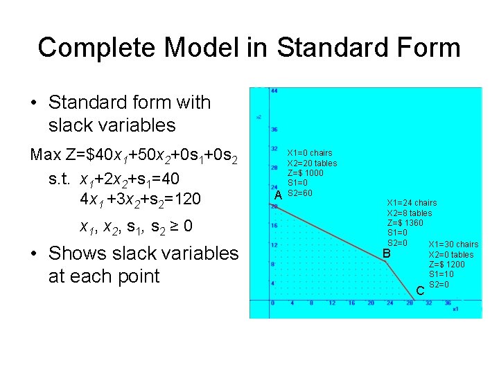
Complete Model in Standard Form • Standard form with slack variables Max Z=$40 x 1+50 x 2+0 s 1+0 s 2 s. t. x 1+2 x 2+s 1=40 4 x 1 +3 x 2+s 2=120 x 1, x 2, s 1, s 2 ≥ 0 • Shows slack variables at each point A X 1=0 chairs X 2=20 tables Z=$ 1000 S 1=0 S 2=60 X 1=24 chairs X 2=8 tables Z=$ 1360 S 1=0 S 2=0 X 1=30 chairs X 2=0 tables B Z=$ 1200 S 1=10 S 2=0 C

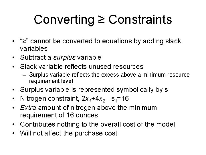
Converting ≥ Constraints • “≥” cannot be converted to equations by adding slack variables • Subtract a surplus variable • Slack variable reflects unused resources – Surplus variable reflects the excess above a minimum resource requirement level • Surplus variable is represented symbolically by s • Nitrogen constraint, 2 x 1+4 x 2 - s 1=16 • Extra amount of nitrogen above the minimum requirement of 16 ounces • Contributes nothing to the overall cost of the model • Will not affect the purchase cost

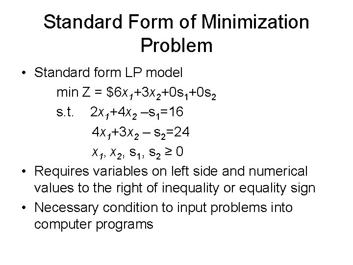
Standard Form of Minimization Problem • Standard form LP model min Z = $6 x 1+3 x 2+0 s 1+0 s 2 s. t. 2 x 1+4 x 2 –s 1=16 4 x 1+3 x 2 – s 2=24 x 1, x 2, s 1, s 2 ≥ 0 • Requires variables on left side and numerical values to the right of inequality or equality sign • Necessary condition to input problems into computer programs

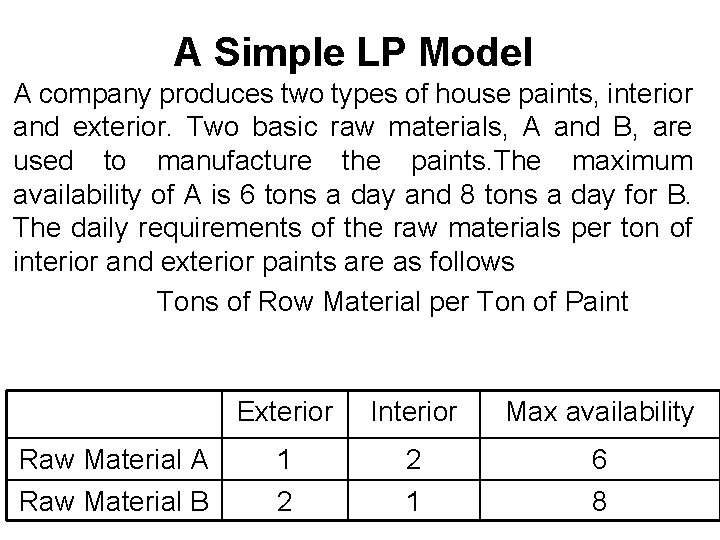
A Simple LP Model A company produces two types of house paints, interior and exterior. Two basic raw materials, A and B, are used to manufacture the paints. The maximum availability of A is 6 tons a day and 8 tons a day for B. The daily requirements of the raw materials per ton of interior and exterior paints are as follows Tons of Row Material per Ton of Paint Raw Material A Raw Material B Exterior Interior Max availability 1 2 2 1 6 8

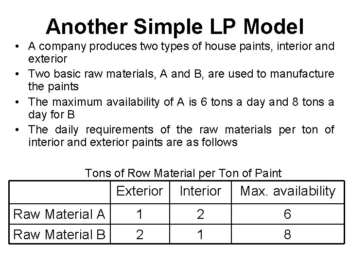
Another Simple LP Model • A company produces two types of house paints, interior and exterior • Two basic raw materials, A and B, are used to manufacture the paints • The maximum availability of A is 6 tons a day and 8 tons a day for B • The daily requirements of the raw materials per ton of interior and exterior paints are as follows Tons of Row Material per Ton of Paint Raw Material A Raw Material B Exterior Interior Max. availability 1 2 2 1 6 8

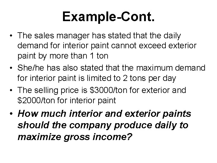
Example-Cont. • The sales manager has stated that the daily demand for interior paint cannot exceed exterior paint by more than 1 ton • She/he has also stated that the maximum demand for interior paint is limited to 2 tons per day • The selling price is $3000/ton for exterior and $2000/ton for interior paint • How much interior and exterior paints should the company produce daily to maximize gross income?

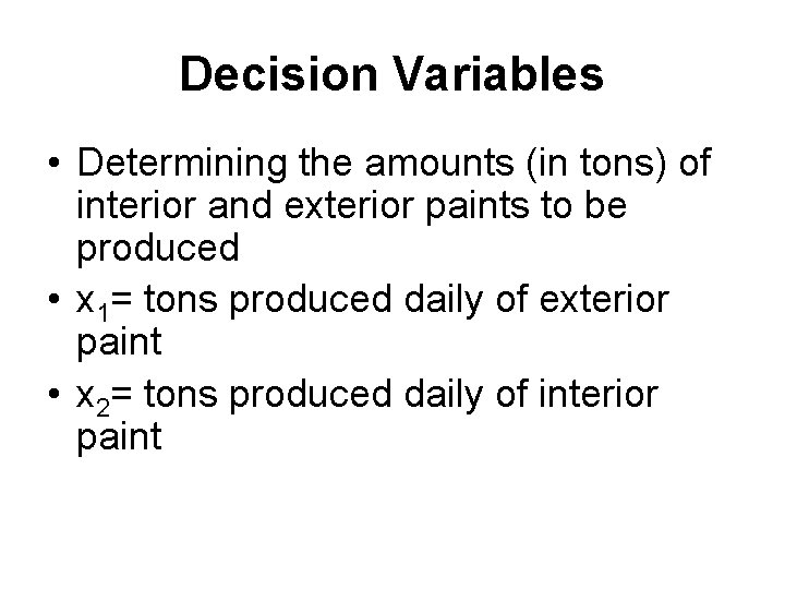
Decision Variables • Determining the amounts (in tons) of interior and exterior paints to be produced • x 1= tons produced daily of exterior paint • x 2= tons produced daily of interior paint

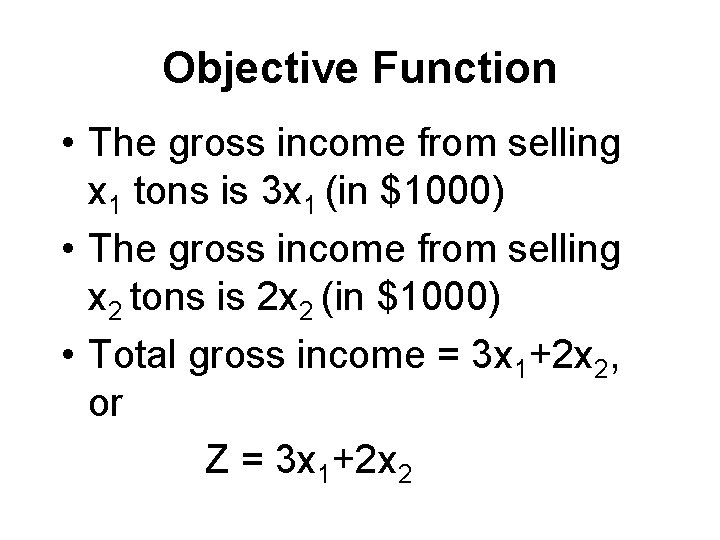
Objective Function • The gross income from selling x 1 tons is 3 x 1 (in $1000) • The gross income from selling x 2 tons is 2 x 2 (in $1000) • Total gross income = 3 x 1+2 x 2, or Z = 3 x 1+2 x 2

Constraints • Constraints impose restrictions on the usage of resources. Three types of restrictions in this example: 1. The usage restriction 2. The demand restriction 3. Nonnegativity restriction

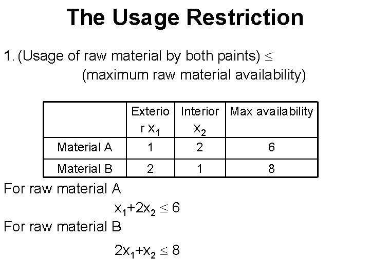
The Usage Restriction 1. (Usage of raw material by both paints) (maximum raw material availability) Exterio Interior Max availability r x 1 x 2 Material A 1 2 6 Material B 2 1 8 For raw material A x 1+2 x 2 6 For raw material B 2 x 1+x 2 8

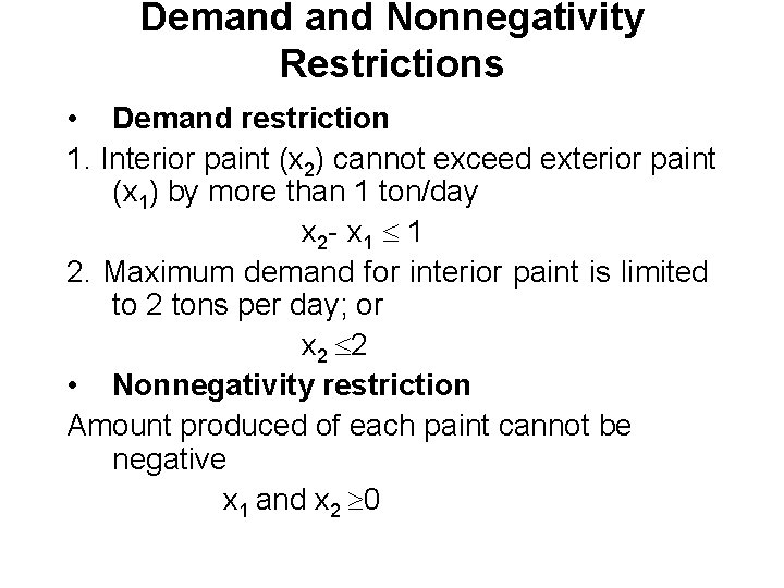
Demand Nonnegativity Restrictions • Demand restriction 1. Interior paint (x 2) cannot exceed exterior paint (x 1) by more than 1 ton/day x 2 - x 1 1 2. Maximum demand for interior paint is limited to 2 tons per day; or x 2 2 • Nonnegativity restriction Amount produced of each paint cannot be negative x 1 and x 2 0

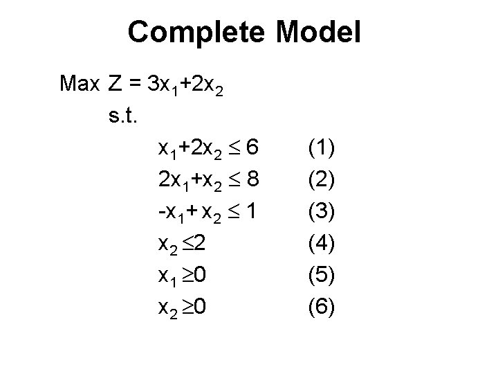
Complete Model Max Z = 3 x 1+2 x 2 s. t. x 1+2 x 2 6 2 x 1+x 2 8 -x 1+ x 2 1 x 2 2 x 1 0 x 2 0 (1) (2) (3) (4) (5) (6)

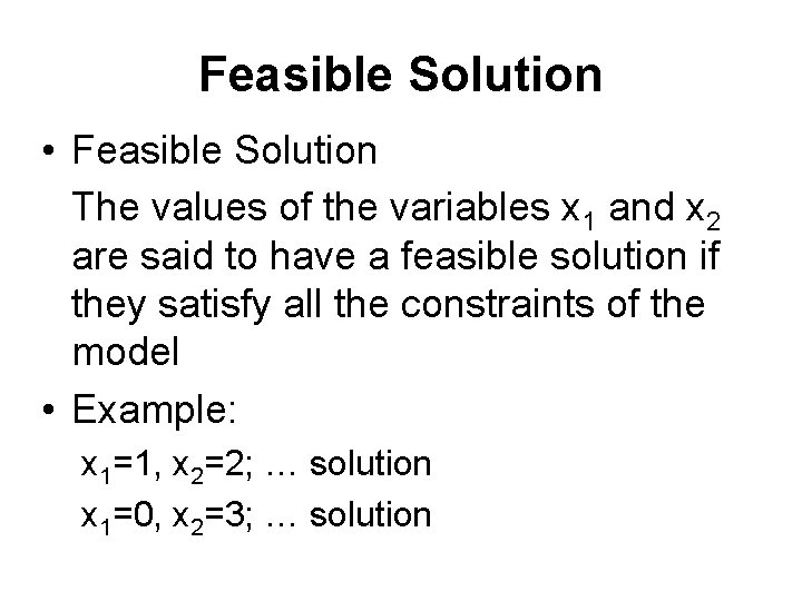
Feasible Solution • Feasible Solution The values of the variables x 1 and x 2 are said to have a feasible solution if they satisfy all the constraints of the model • Example: x 1=1, x 2=2; … solution x 1=0, x 2=3; … solution

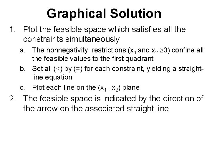
Graphical Solution 1. Plot the feasible space which satisfies all the constraints simultaneously a. The nonnegativity restrictions (x 1 and x 2 0) confine all the feasible values to the first quadrant b. Set all ( ) by (=) for each constraint, yielding a straightline equation c. Plot each line on the (x 1 , x 2) plane 2. The feasible space is indicated by the direction of the arrow on the associated straight line

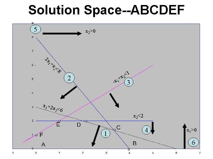
Solution Space--ABCDEF 5 x 2>0 2 x 1+ x 2< 8 <1 2 x x 1+ 2 - 3 x 1 +2 x 2 <6 x 2<2 1 4 x 1>0 6

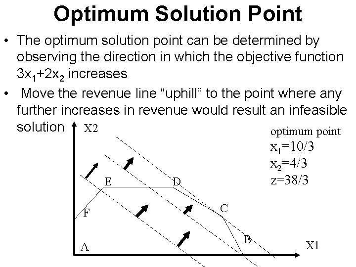
Optimum Solution Point • The optimum solution point can be determined by observing the direction in which the objective function 3 x 1+2 x 2 increases • Move the revenue line “uphill” to the point where any further increases in revenue would result an infeasible solution X 2 optimum point x 1=10/3 x 2=4/3 z=38/3 E D F A C B X 1

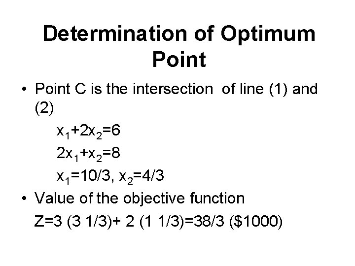
Determination of Optimum Point • Point C is the intersection of line (1) and (2) x 1+2 x 2=6 2 x 1+x 2=8 x 1=10/3, x 2=4/3 • Value of the objective function Z=3 (3 1/3)+ 2 (1 1/3)=38/3 ($1000)

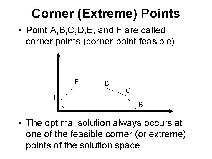
Corner (Extreme) Points • Point A, B, C, D, E, and F are called corner points (corner-point feasible) E F A D C B • The optimal solution always occurs at one of the feasible corner (or extreme) points of the solution space

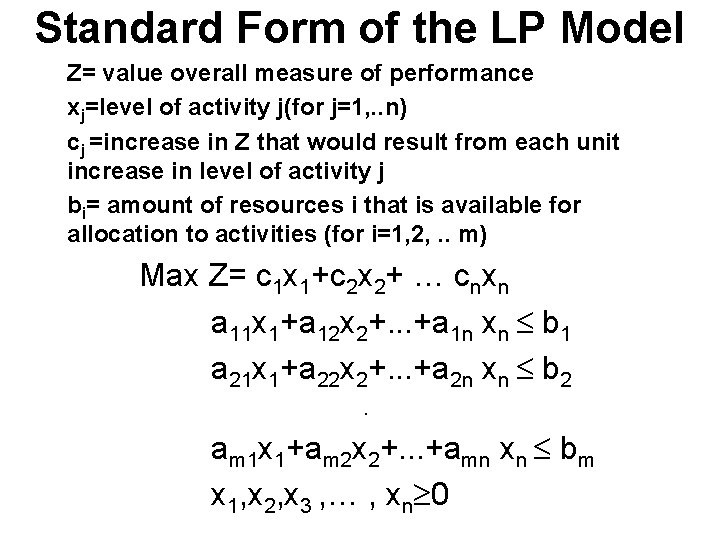
Standard Form of the LP Model Z= value overall measure of performance xj=level of activity j(for j=1, . . n) cj =increase in Z that would result from each unit increase in level of activity j bi= amount of resources i that is available for allocation to activities (for i=1, 2, . . m) Max Z= c 1 x 1+c 2 x 2+ … cnxn a 11 x 1+a 12 x 2+. . . +a 1 n xn b 1 a 21 x 1+a 22 x 2+. . . +a 2 n xn b 2. am 1 x 1+am 2 x 2+. . . +amn xn bm x 1, x 2, x 3 , … , xn 0

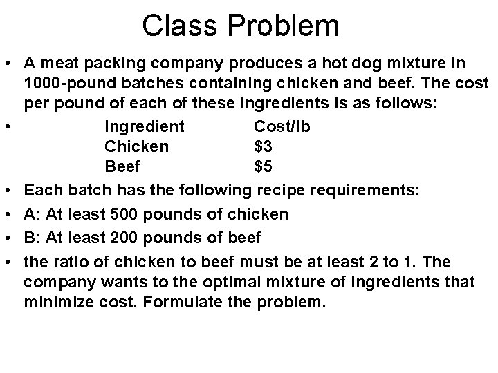
Class Problem • A meat packing company produces a hot dog mixture in 1000 -pound batches containing chicken and beef. The cost per pound of each of these ingredients is as follows: • Ingredient Cost/lb Chicken $3 Beef $5 • Each batch has the following recipe requirements: • A: At least 500 pounds of chicken • B: At least 200 pounds of beef • the ratio of chicken to beef must be at least 2 to 1. The company wants to the optimal mixture of ingredients that minimize cost. Formulate the problem.

Complete Model • Identify the decision variables • Formulate the obj fcn as Min z=… +… • Establish model constraints as … … …

Summary • Provided you with a good start in LP modeling • Learned how to formulate two simple LP models, a maximization and a minimization problem • Showed how to use the graphical approach to find optimal solution point and how to put a linear programming model in the standard format

HW Assignments • Problem set 2. 1 A: prob. 2. Problem Set 2. 2 A: Prob. 5, 11 and 12 Problem set 2. 2 B: prob. 4. Problem set 3. 1 A: prob. 1 and prob. 2. • Problem set 3. 6 A: Problem 2. Problem set 3. 6 B: Problem 3. Problem set 2. 3 D: Problem 3. These problems can be solved using either by Solver or TORA.