Chapter 2 Graphing Equations and Inequalities Chapter Sections

Chapter 2 Graphing Equations and Inequalities

Chapter Sections 2. 1 – Reading Graphs and the Rectangular Coordinate System 2. 2 – Graphing Linear Equations 2. 3 – Intercepts 2. 4 – Slope and Rate of Change 2. 5 – Equations of Lines 2. 6 – Introduction to Functions 2. 7 – Graphing Linear Inequalities in Two Variables 2. 8 – Direct and Inverse Variation 2

§ 2. 1 Reading Graphs and the Rectangular Coordinate System

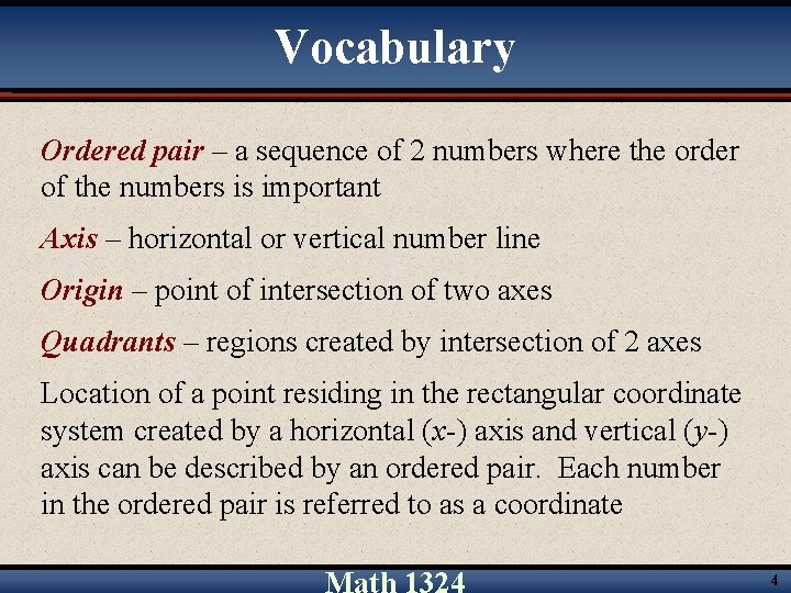
Vocabulary Ordered pair – a sequence of 2 numbers where the order of the numbers is important Axis – horizontal or vertical number line Origin – point of intersection of two axes Quadrants – regions created by intersection of 2 axes Location of a point residing in the rectangular coordinate system created by a horizontal (x-) axis and vertical (y-) axis can be described by an ordered pair. Each number in the ordered pair is referred to as a coordinate 4

Graphing an Ordered Pair To graph the point corresponding to a particular ordered pair (a, b), you must start at the origin and move a units to the left of right (right if a is positive, left if a is negative), then move b units up or down (up if b is positive, down if b is negative). 5

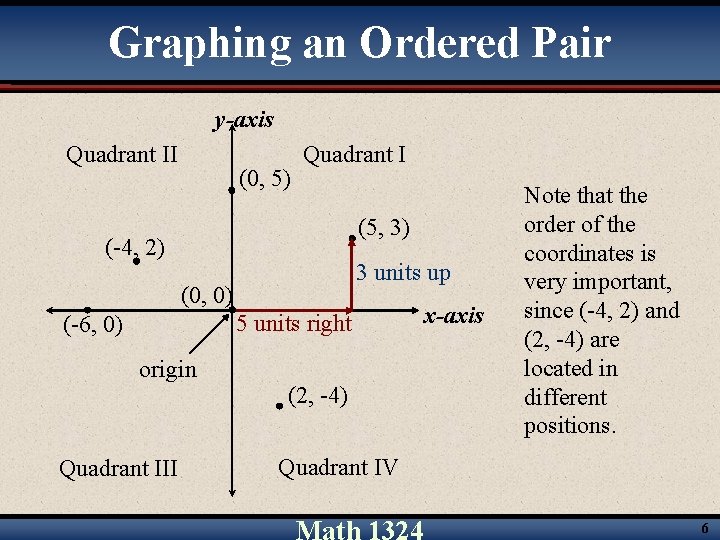
Graphing an Ordered Pair y-axis Quadrant II (0, 5) Quadrant I (5, 3) (-4, 2) 3 units up (0, 0) 5 units right (-6, 0) origin Quadrant III (2, -4) x-axis Note that the order of the coordinates is very important, since (-4, 2) and (2, -4) are located in different positions. Quadrant IV 6

Vocabulary Paired data are data that can be represented as an ordered pair A scatter diagram is the graph of paired data as points in the rectangular coordinate system An order pair is a solution of an equation in two variables if replacing the variables by the appropriate values of the ordered pair results in a true statement. 7

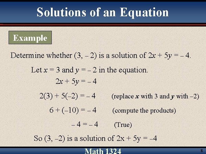
Solutions of an Equation Example Determine whether (3, – 2) is a solution of 2 x + 5 y = – 4. Let x = 3 and y = – 2 in the equation. 2 x + 5 y = – 4 2(3) + 5(– 2) = – 4 6 + (– 10) = – 4=– 4 (replace x with 3 and y with – 2) (compute the products) (True) So (3, – 2) is a solution of 2 x + 5 y = – 4 8

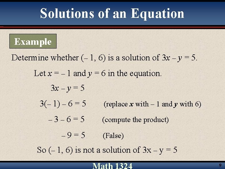
Solutions of an Equation Example Determine whether (– 1, 6) is a solution of 3 x – y = 5. Let x = – 1 and y = 6 in the equation. 3 x – y = 5 3(– 1) – 6 = 5 – 3– 6=5 – 9=5 (replace x with – 1 and y with 6) (compute the product) (False) So (– 1, 6) is not a solution of 3 x – y = 5 9

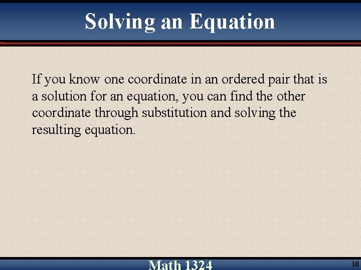
Solving an Equation If you know one coordinate in an ordered pair that is a solution for an equation, you can find the other coordinate through substitution and solving the resulting equation. 10

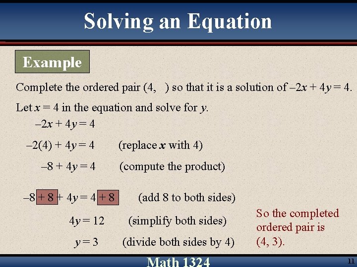
Solving an Equation Example Complete the ordered pair (4, ) so that it is a solution of – 2 x + 4 y = 4. Let x = 4 in the equation and solve for y. – 2 x + 4 y = 4 – 2(4) + 4 y = 4 – 8 + 8 + 4 y = 4 + 8 (replace x with 4) (compute the product) (add 8 to both sides) 4 y = 12 (simplify both sides) y=3 (divide both sides by 4) So the completed ordered pair is (4, 3). 11

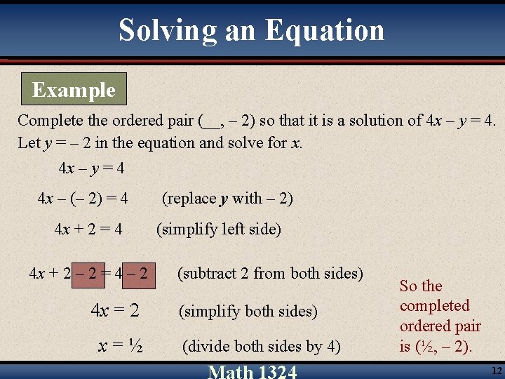
Solving an Equation Example Complete the ordered pair (__, – 2) so that it is a solution of 4 x – y = 4. Let y = – 2 in the equation and solve for x. 4 x – y = 4 4 x – (– 2) = 4 4 x + 2 – 2 = 4 – 2 4 x = 2 x=½ (replace y with – 2) (simplify left side) (subtract 2 from both sides) (simplify both sides) (divide both sides by 4) So the completed ordered pair is (½, – 2). 12

§ 2. 2 Graphing Linear Equations

Linear Equations Linear Equation in Two Variables Ax + By = C A, B, C are real numbers, A and B not both 0 This is called “standard form” Graphing Linear Equations Find at least 2 points on the line y = mx + b crosses the y-axis at b (called “slopeintercept form”) 14

Graphing Linear Equations Example Graph the linear equation 2 x – y = – 4. We find two ordered pair solutions (and a third solution as a check on our computations) by choosing a value for one of the variables, x or y, then solving for the other variable. We plot the solution points, then draw the line containing the 3 points. Continued. 15

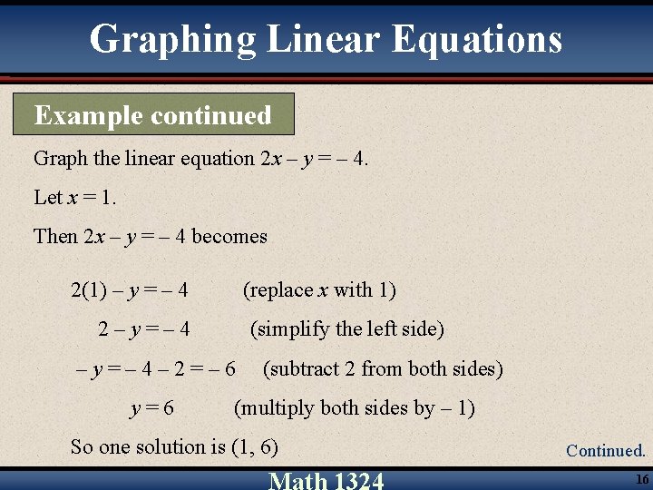
Graphing Linear Equations Example continued Graph the linear equation 2 x – y = – 4. Let x = 1. Then 2 x – y = – 4 becomes 2(1) – y = – 4 (replace x with 1) 2–y=– 4 (simplify the left side) –y=– 4– 2=– 6 y=6 (subtract 2 from both sides) (multiply both sides by – 1) So one solution is (1, 6) Continued. 16

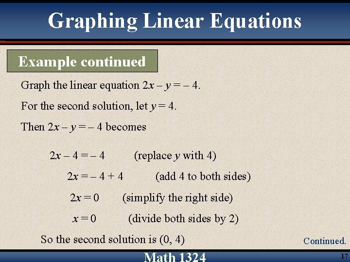
Graphing Linear Equations Example continued Graph the linear equation 2 x – y = – 4. For the second solution, let y = 4. Then 2 x – y = – 4 becomes 2 x – 4 = – 4 (replace y with 4) 2 x = – 4 + 4 2 x = 0 x=0 (add 4 to both sides) (simplify the right side) (divide both sides by 2) So the second solution is (0, 4) Continued. 17

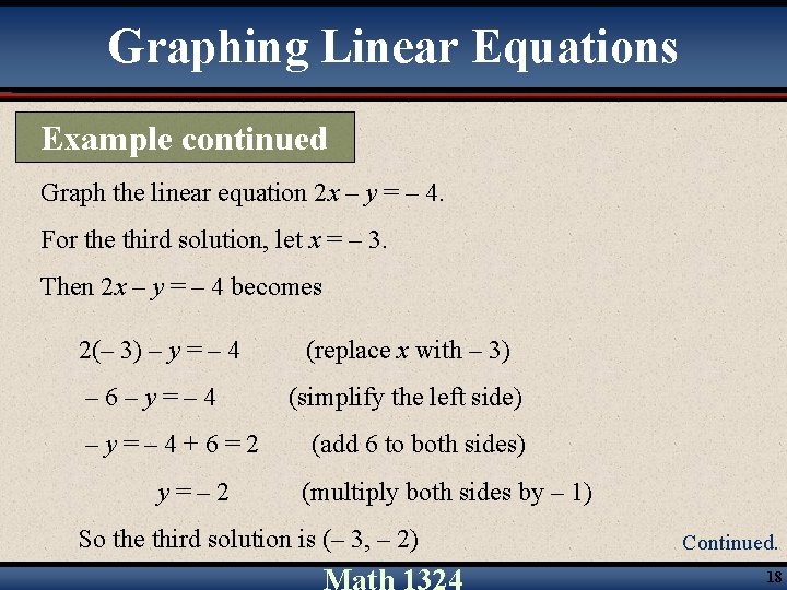
Graphing Linear Equations Example continued Graph the linear equation 2 x – y = – 4. For the third solution, let x = – 3. Then 2 x – y = – 4 becomes 2(– 3) – y = – 4 – 6–y=– 4+6=2 y=– 2 (replace x with – 3) (simplify the left side) (add 6 to both sides) (multiply both sides by – 1) So the third solution is (– 3, – 2) Continued. 18

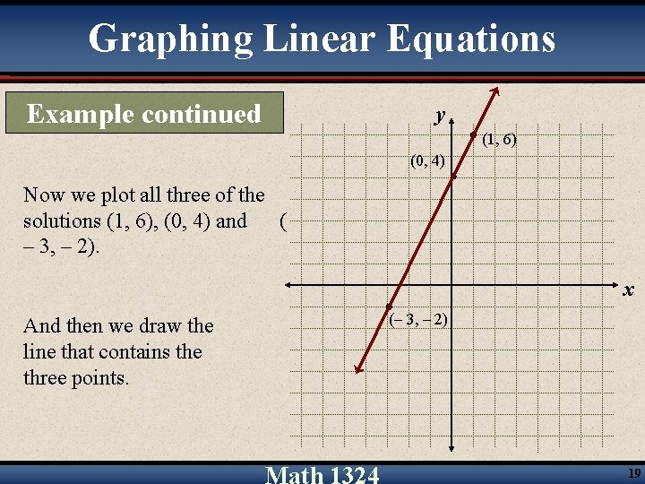
Graphing Linear Equations Example continued y (1, 6) (0, 4) Now we plot all three of the solutions (1, 6), (0, 4) and ( – 3, – 2). x And then we draw the line that contains the three points. (– 3, – 2) 19

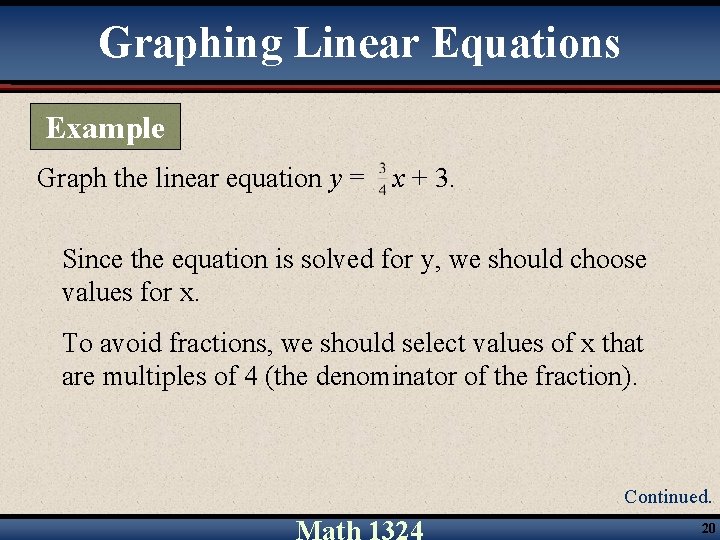
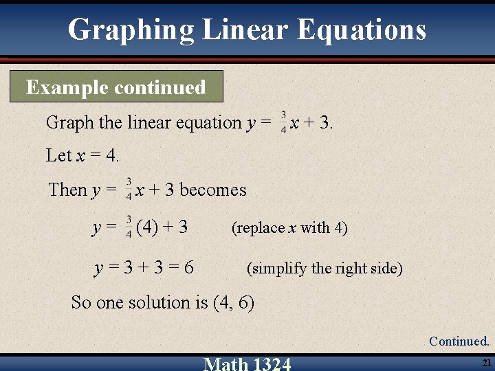
Graphing Linear Equations Example Graph the linear equation y = x + 3. Since the equation is solved for y, we should choose values for x. To avoid fractions, we should select values of x that are multiples of 4 (the denominator of the fraction). Continued. 20

Graphing Linear Equations Example continued Graph the linear equation y = x + 3. Let x = 4. Then y = x + 3 becomes y = (4) + 3 y=3+3=6 (replace x with 4) (simplify the right side) So one solution is (4, 6) Continued. 21

Graphing Linear Equations Example continued Graph the linear equation y = x + 3. For the second solution, let x = 0. Then y = y= x + 3 becomes (0) + 3 y=0+3=3 (replace x with 0) (simplify the right side) So a second solution is (0, 3) Continued. 22

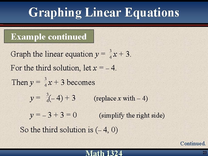
Graphing Linear Equations Example continued Graph the linear equation y = x + 3. For the third solution, let x = – 4. Then y = y= x + 3 becomes (– 4) + 3 y=– 3+3=0 (replace x with – 4) (simplify the right side) So the third solution is (– 4, 0) Continued. 23

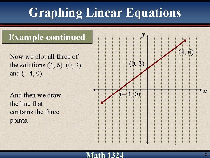
Graphing Linear Equations y Example continued Now we plot all three of the solutions (4, 6), (0, 3) and (– 4, 0). And then we draw the line that contains the three points. (4, 6) (0, 3) (– 4, 0) x 24

§ 2. 3 Intercepts

Intercepts of axes (where graph crosses the axes) Since all points on the x-axis have a y-coordinate of 0, to find x-intercept, let y = 0 and solve for x Since all points on the y-axis have an x-coordinate of 0, to find y-intercept, let x = 0 and solve for y 26

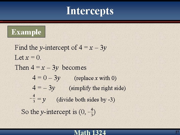
Intercepts Example Find the y-intercept of 4 = x – 3 y Let x = 0. Then 4 = x – 3 y becomes 4 = 0 – 3 y (replace x with 0) 4 = – 3 y (simplify the right side) =y (divide both sides by -3) So the y-intercept is (0, ) 27

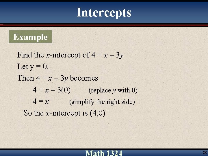
Intercepts Example Find the x-intercept of 4 = x – 3 y Let y = 0. Then 4 = x – 3 y becomes 4 = x – 3(0) (replace y with 0) 4=x (simplify the right side) So the x-intercept is (4, 0) 28

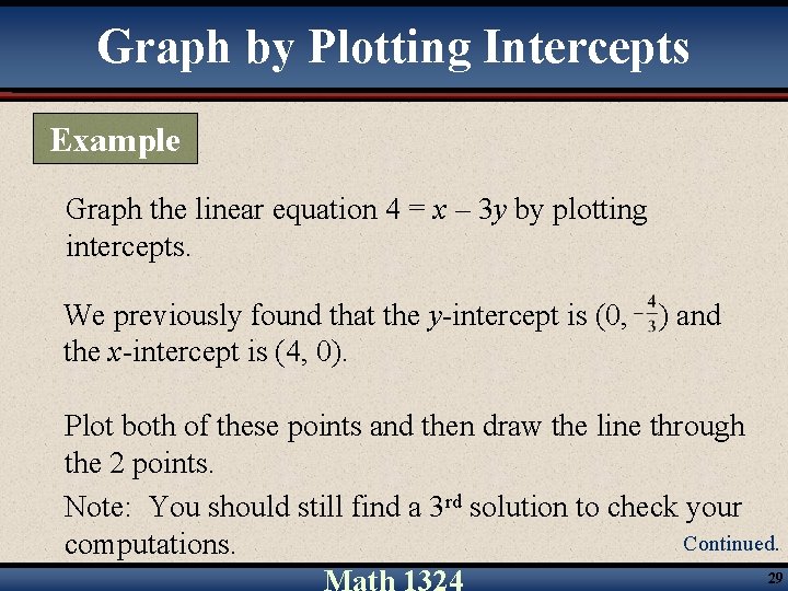
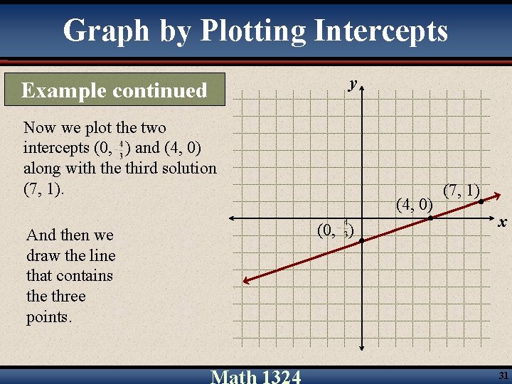
Graph by Plotting Intercepts Example Graph the linear equation 4 = x – 3 y by plotting intercepts. We previously found that the y-intercept is (0, the x-intercept is (4, 0). ) and Plot both of these points and then draw the line through the 2 points. Note: You should still find a 3 rd solution to check your Continued. computations. 29

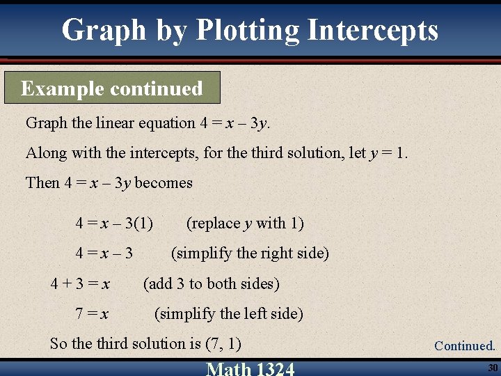
Graph by Plotting Intercepts Example continued Graph the linear equation 4 = x – 3 y. Along with the intercepts, for the third solution, let y = 1. Then 4 = x – 3 y becomes 4 = x – 3(1) 4=x– 3 4+3=x 7=x (replace y with 1) (simplify the right side) (add 3 to both sides) (simplify the left side) So the third solution is (7, 1) Continued. 30

Graph by Plotting Intercepts Example continued y Now we plot the two intercepts (0, ) and (4, 0) along with the third solution (7, 1). And then we draw the line that contains the three points. (4, 0) (0, ) (7, 1) x 31

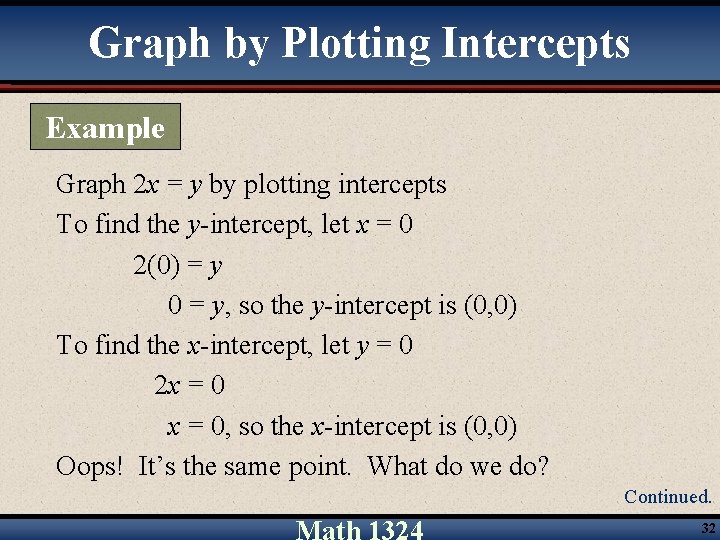
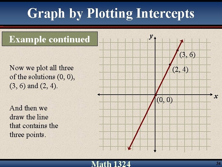
Graph by Plotting Intercepts Example Graph 2 x = y by plotting intercepts To find the y-intercept, let x = 0 2(0) = y 0 = y, so the y-intercept is (0, 0) To find the x-intercept, let y = 0 2 x = 0, so the x-intercept is (0, 0) Oops! It’s the same point. What do we do? Continued. 32

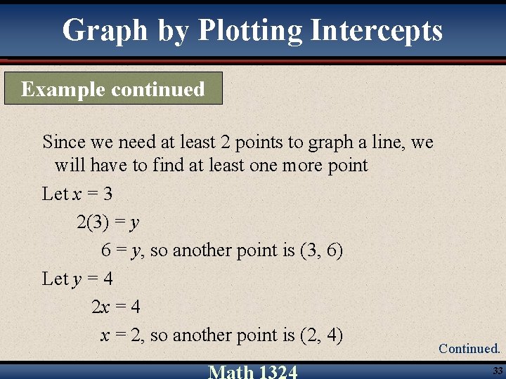
Graph by Plotting Intercepts Example continued Since we need at least 2 points to graph a line, we will have to find at least one more point Let x = 3 2(3) = y 6 = y, so another point is (3, 6) Let y = 4 2 x = 4 x = 2, so another point is (2, 4) Continued. 33

Graph by Plotting Intercepts Example continued y (3, 6) Now we plot all three of the solutions (0, 0), (3, 6) and (2, 4). And then we draw the line that contains the three points. (2, 4) (0, 0) x 34

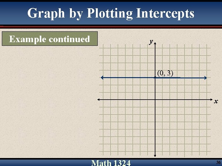
Graph by Plotting Intercepts Example Graph y = 3 Note that this line can be written as y = 0·x + 3 The y-intercept is (0, 3), but there is no x-intercept! (Since an x-intercept would be found by letting y = 0, and 0 0·x + 3, there is no x-intercept) Every value we substitute for x gives a y-coordinate of 3 The graph will be a horizontal line through the point (0, 3) on the y-axis Continued. 35

Graph by Plotting Intercepts Example continued y (0, 3) x 36

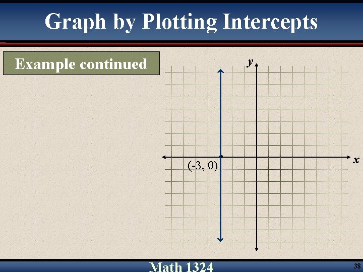
Graph by Plotting Intercepts Example Graph x = – 3 This equation can be written x = 0·y – 3 When y = 0, x = – 3, so the x-intercept is (– 3, 0), but there is no y-intercept Any value we substitute for y gives an x-coordinate of – 3 So the graph will be a vertical line through the point (– 3, 0) on the x-axis Continued. 37

Graph by Plotting Intercepts y Example continued (-3, 0) x 38

Vertical and Horizontal Lines Vertical lines Appear in the form of x = c, where c is a real number x-intercept is at (c, 0), no y-intercept unless c = 0 (y-axis) Horizontal lines Appear in the form of y = c, where c is a real number y-intercept is at (0, c), no x-intercept unless c = 0 (x-axis) 39

§ 2. 4 Slope and Rate of Change

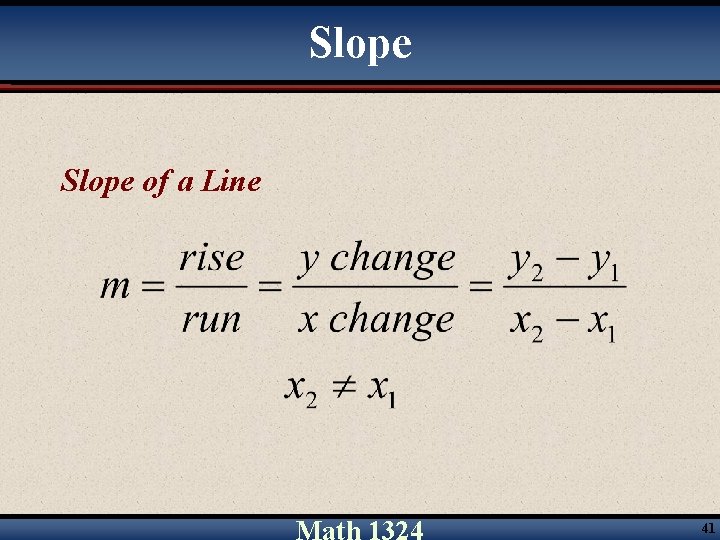
Slope of a Line 41

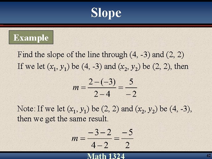
Slope Example Find the slope of the line through (4, -3) and (2, 2) If we let (x 1, y 1) be (4, -3) and (x 2, y 2) be (2, 2), then Note: If we let (x 1, y 1) be (2, 2) and (x 2, y 2) be (4, -3), then we get the same result. 42

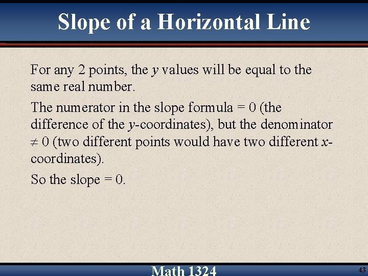
Slope of a Horizontal Line For any 2 points, the y values will be equal to the same real number. The numerator in the slope formula = 0 (the difference of the y-coordinates), but the denominator 0 (two different points would have two different xcoordinates). So the slope = 0. 43

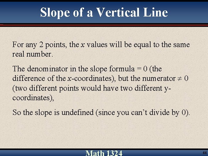
Slope of a Vertical Line For any 2 points, the x values will be equal to the same real number. The denominator in the slope formula = 0 (the difference of the x-coordinates), but the numerator 0 (two different points would have two different ycoordinates), So the slope is undefined (since you can’t divide by 0). 44

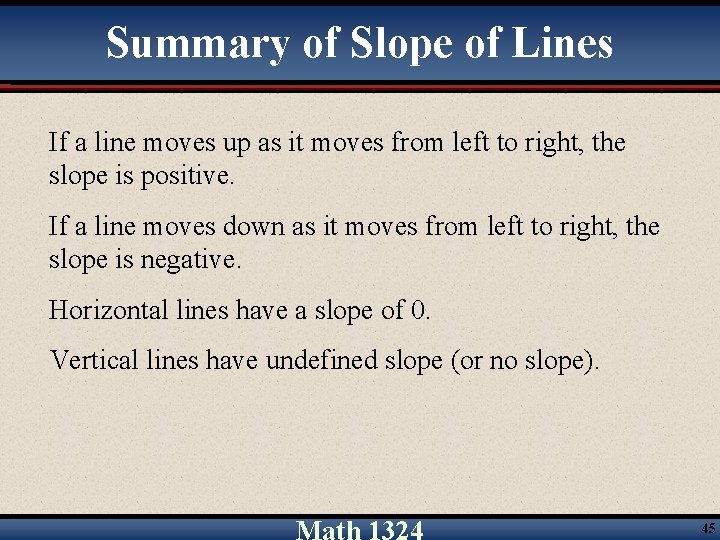
Summary of Slope of Lines If a line moves up as it moves from left to right, the slope is positive. If a line moves down as it moves from left to right, the slope is negative. Horizontal lines have a slope of 0. Vertical lines have undefined slope (or no slope). 45

Parallel Lines Two lines that never intersect are called parallel lines. Parallel lines have the same slope • unless they are vertical lines, which have no slope. Vertical lines are also parallel. 46

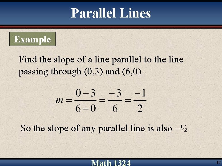
Parallel Lines Example Find the slope of a line parallel to the line passing through (0, 3) and (6, 0) So the slope of any parallel line is also –½ 47

Perpendicular Lines Two lines that intersect at right angles are called perpendicular lines Two nonvertical perpendicular lines have slopes that are negative reciprocals of each other The product of their slopes will be – 1 Horizontal and vertical lines are perpendicular to each other 48

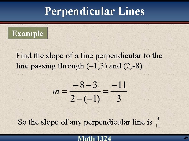
Perpendicular Lines Example Find the slope of a line perpendicular to the line passing through ( 1, 3) and (2, -8) So the slope of any perpendicular line is 49

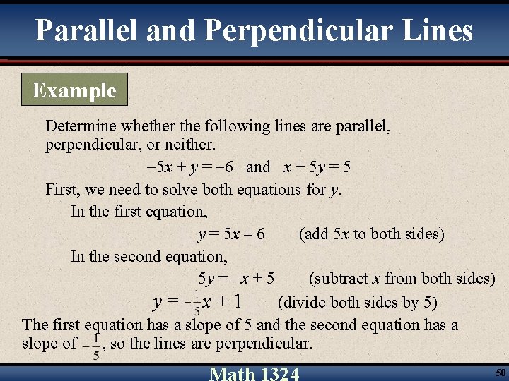
Parallel and Perpendicular Lines Example Determine whether the following lines are parallel, perpendicular, or neither. 5 x + y = 6 and x + 5 y = 5 First, we need to solve both equations for y. In the first equation, y = 5 x – 6 (add 5 x to both sides) In the second equation, 5 y = x + 5 (subtract x from both sides) y= x+1 (divide both sides by 5) The first equation has a slope of 5 and the second equation has a slope of , so the lines are perpendicular. 50

§ 2. 5 Equations of Lines

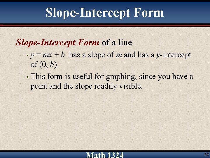
Slope-Intercept Form of a line y = mx + b has a slope of m and has a y-intercept of (0, b). • This form is useful for graphing, since you have a point and the slope readily visible. • 52

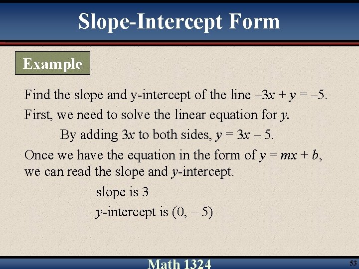
Slope-Intercept Form Example Find the slope and y-intercept of the line – 3 x + y = – 5. First, we need to solve the linear equation for y. By adding 3 x to both sides, y = 3 x – 5. Once we have the equation in the form of y = mx + b, we can read the slope and y-intercept. slope is 3 y-intercept is (0, – 5) 53

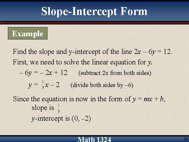
Slope-Intercept Form Example Find the slope and y-intercept of the line 2 x – 6 y = 12. First, we need to solve the linear equation for y. – 6 y = – 2 x + 12 (subtract 2 x from both sides) y= x– 2 (divide both sides by – 6) Since the equation is now in the form of y = mx + b, slope is y-intercept is (0, – 2) 54

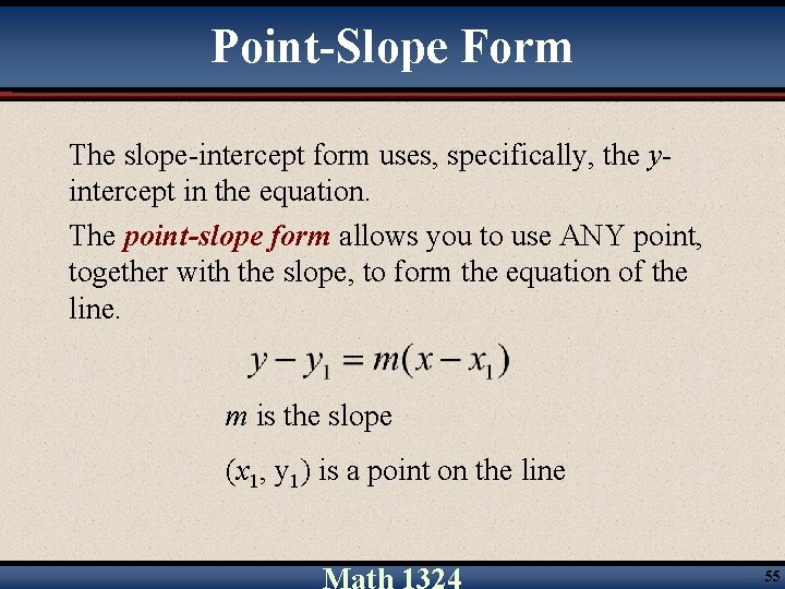
Point-Slope Form The slope-intercept form uses, specifically, the yintercept in the equation. The point-slope form allows you to use ANY point, together with the slope, to form the equation of the line. m is the slope (x 1, y 1) is a point on the line 55

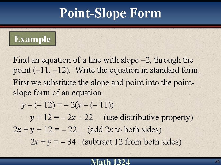
Point-Slope Form Example Find an equation of a line with slope – 2, through the point (– 11, – 12). Write the equation in standard form. First we substitute the slope and point into the pointslope form of an equation. y – (– 12) = – 2(x – (– 11)) y + 12 = – 2 x – 22 (use distributive property) 2 x + y + 12 = – 22 (add 2 x to both sides) 2 x + y = – 34 (subtract 12 from both sides) 56

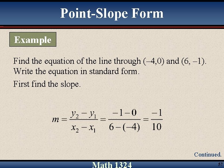
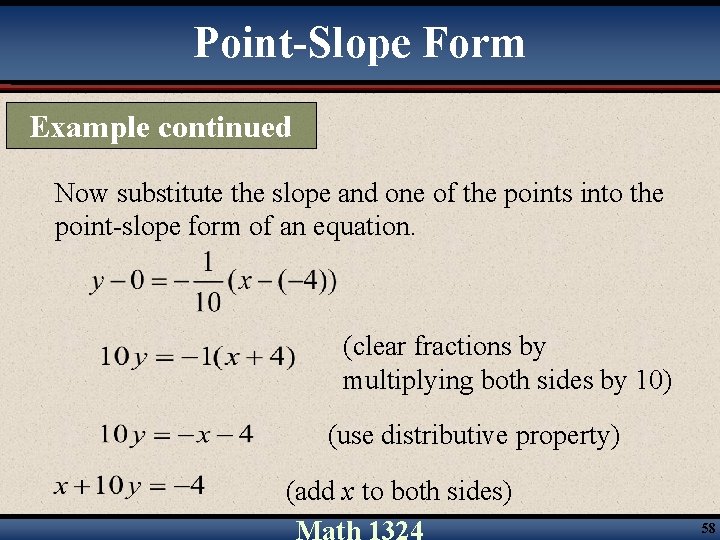
Point-Slope Form Example Find the equation of the line through (– 4, 0) and (6, – 1). Write the equation in standard form. First find the slope. Continued. 57

Point-Slope Form Example continued Now substitute the slope and one of the points into the point-slope form of an equation. (clear fractions by multiplying both sides by 10) (use distributive property) (add x to both sides) 58

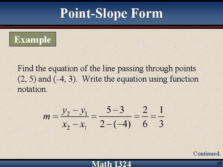
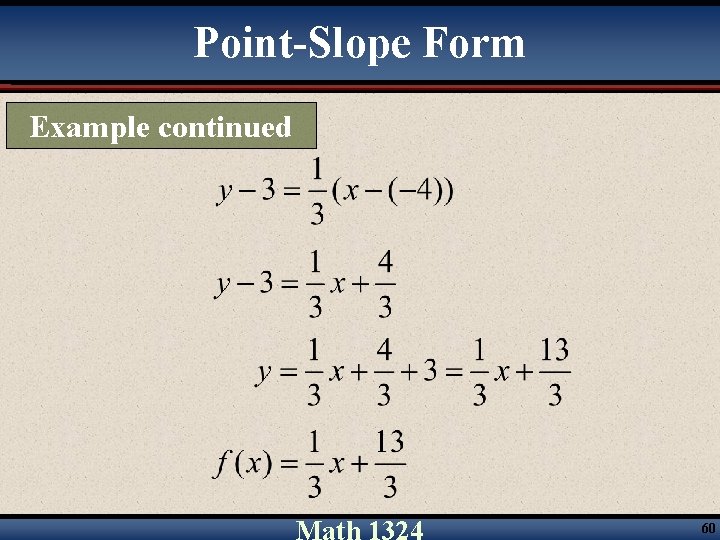
Point-Slope Form Example Find the equation of the line passing through points (2, 5) and (– 4, 3). Write the equation using function notation. Continued. 59

Point-Slope Form Example continued 60

§ 2. 6 Introduction to Functions

Vocabulary • An equation in 2 variables defines a relation between the two variables. • A set of ordered pairs is also called a relation. • The domain is the set of x-coordinates of the ordered pairs • The range is the set of y-coordinates of the ordered pairs 62

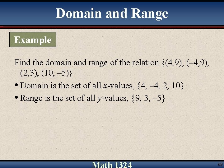
Domain and Range Example Find the domain and range of the relation {(4, 9), (– 4, 9), (2, 3), (10, – 5)} • Domain is the set of all x-values, {4, – 4, 2, 10} • Range is the set of all y-values, {9, 3, – 5} 63

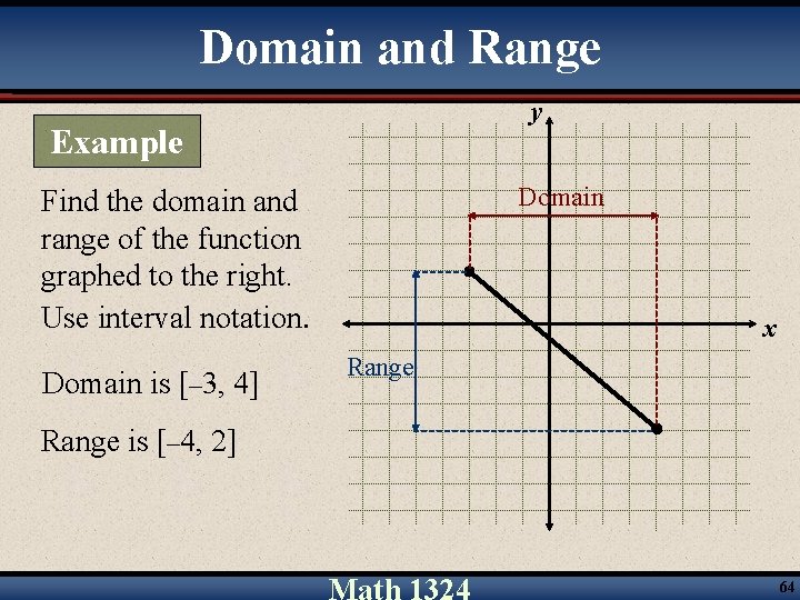
Domain and Range y Example Domain Find the domain and range of the function graphed to the right. Use interval notation. Domain is [– 3, 4] x Range is [– 4, 2] 64

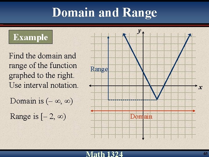
Domain and Range y Example Find the domain and range of the function graphed to the right. Use interval notation. Range x Domain is (– , ) Range is [– 2, ) Domain 65

Functions Some relations are also functions. A function is a set of order pairs that assigns to each x-value exactly one y-value. 66

Functions Example Given the relation {(4, 9), (– 4, 9), (2, 3), (10, – 5)}, is it a function? Since each element of the domain is paired with only one element of the range, it is a function. Note: It’s okay for a y-value to be assigned to more than one x-value, but an x-value cannot be assigned to more than one y-value (has to be assigned to ONLY one y-value). 67

Vertical Line Test • Relations and functions can also be described by graphing their ordered pairs. • Graphs can be used to determine if a relation is a function. • If an x-coordinate is paired with more than one ycoordinate, a vertical line can be drawn that will intersect the graph at more than one point. • If no vertical line can be drawn so that it intersects a graph more than once, the graph is the graph of a function. This is the vertical line test. 68

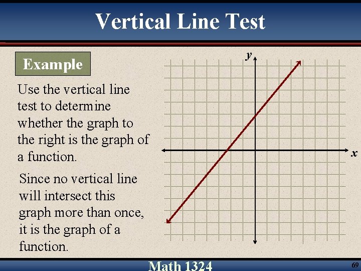
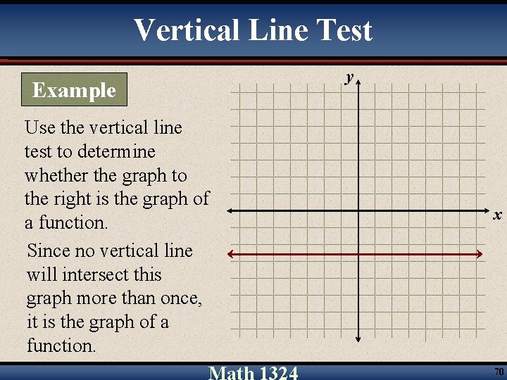
Vertical Line Test Example Use the vertical line test to determine whether the graph to the right is the graph of a function. y x Since no vertical line will intersect this graph more than once, it is the graph of a function. 69

Vertical Line Test Example Use the vertical line test to determine whether the graph to the right is the graph of a function. Since no vertical line will intersect this graph more than once, it is the graph of a function. y x 70

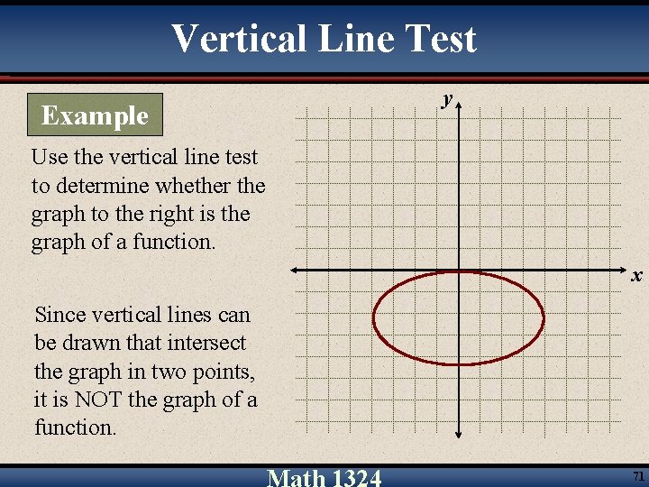
Vertical Line Test Example y Use the vertical line test to determine whether the graph to the right is the graph of a function. x Since vertical lines can be drawn that intersect the graph in two points, it is NOT the graph of a function. 71

Vertical Line Test Since the graph of a linear equation is a line, all linear equations are functions, except those whose graph is a vertical line Note: An equation of the form y = c is a horizontal line and IS a function. An equation of the form x = c is a vertical line and IS NOT a function. 72

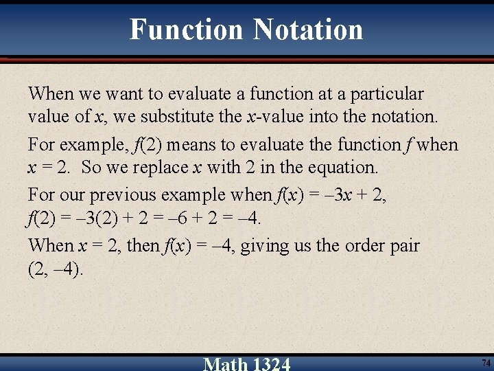
Function Notation • Specialized notation is often used when we know a relation is a function and it has been solved for y. • For example, the graph of the linear equation y = – 3 x + 2 passes the vertical line test, so it represents a function. • We often use letters such as f, g, and h to name functions. • We can use the function notation f(x) (read “f of x”) and write the equation as f(x) = – 3 x + 2. Note: The symbol f(x) is a specialized notation that does NOT mean f • x (f times x). 73

Function Notation When we want to evaluate a function at a particular value of x, we substitute the x-value into the notation. For example, f(2) means to evaluate the function f when x = 2. So we replace x with 2 in the equation. For our previous example when f(x) = – 3 x + 2, f(2) = – 3(2) + 2 = – 6 + 2 = – 4. When x = 2, then f(x) = – 4, giving us the order pair (2, – 4). 74

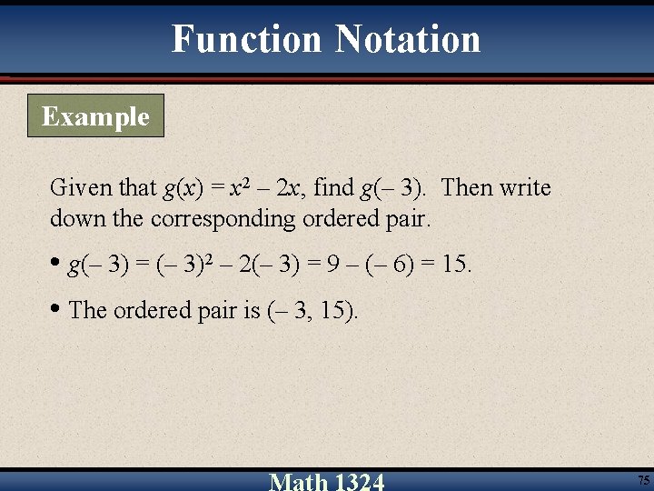
Function Notation Example Given that g(x) = x 2 – 2 x, find g(– 3). Then write down the corresponding ordered pair. • g(– 3) = (– 3)2 – 2(– 3) = 9 – (– 6) = 15. • The ordered pair is (– 3, 15). 75

§ 2. 7 Graphing Linear Inequalities in Two Variables

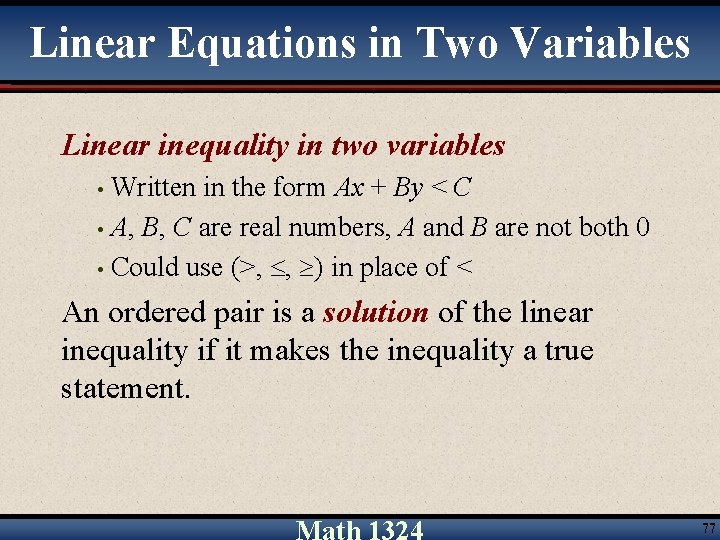
Linear Equations in Two Variables Linear inequality in two variables Written in the form Ax + By < C • A, B, C are real numbers, A and B are not both 0 • Could use (>, , ) in place of < • An ordered pair is a solution of the linear inequality if it makes the inequality a true statement. 77

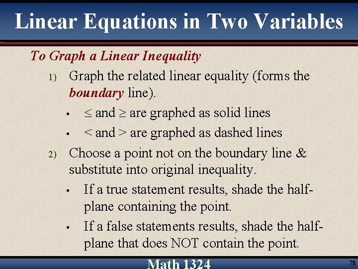
Linear Equations in Two Variables To Graph a Linear Inequality 1) Graph the related linear equality (forms the boundary line). • and are graphed as solid lines • < and > are graphed as dashed lines 2) Choose a point not on the boundary line & substitute into original inequality. • If a true statement results, shade the halfplane containing the point. • If a false statements results, shade the halfplane that does NOT contain the point. 78

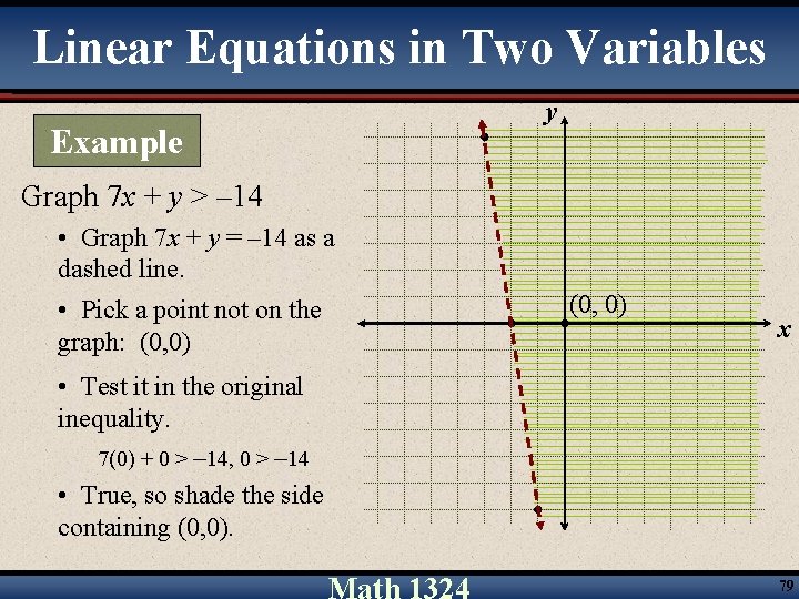
Linear Equations in Two Variables Example y Graph 7 x + y > – 14 • Graph 7 x + y = – 14 as a dashed line. • Pick a point not on the graph: (0, 0) x • Test it in the original inequality. 7(0) + 0 > – 14, 0 > – 14 • True, so shade the side containing (0, 0). 79

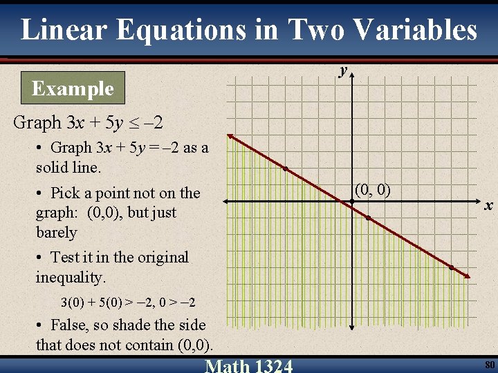
Linear Equations in Two Variables Example y Graph 3 x + 5 y – 2 • Graph 3 x + 5 y = – 2 as a solid line. • Pick a point not on the graph: (0, 0), but just barely • Test it in the original inequality. 3(0) + 5(0) > – 2, 0 > – 2 • False, so shade the side that does not contain (0, 0) x 80

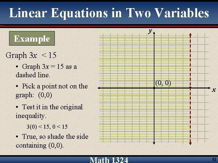
Linear Equations in Two Variables Example y Graph 3 x < 15 • Graph 3 x = 15 as a dashed line. • Pick a point not on the graph: (0, 0) x • Test it in the original inequality. 3(0) < 15, 0 < 15 • True, so shade the side containing (0, 0). 81

Linear Equations in Two Variables Warning! Note that although all of our examples allowed us to select (0, 0) as our test point, that will not always be true. If the boundary line contains (0, 0), you must select another point that is not contained on the line as your test point. 82

§ 2. 8 Direct and Inverse Variation

Direct Variation y varies directly as x, or y is directly proportional to x, if there is a nonzero constant k such that y = kx. The family of equations of the form y = kx are referred to as direct variation equations. The number k is called the constant of variation or the constant of proportionality. 84

Direct Variation If y varies directly as x, find the constant of variation k and the direct variation equation, given that y = 5 when x = 30. y = kx 5 = k· 30 k = 1/6 1 So the direct variation equation is y = x 6 85

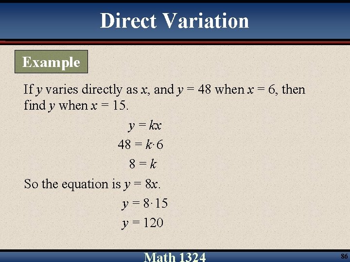
Direct Variation Example If y varies directly as x, and y = 48 when x = 6, then find y when x = 15. y = kx 48 = k· 6 8=k So the equation is y = 8 x. y = 8· 15 y = 120 86

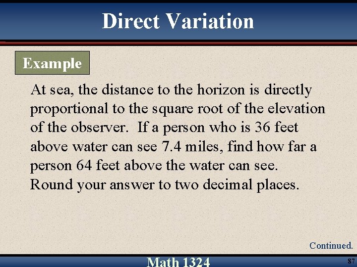
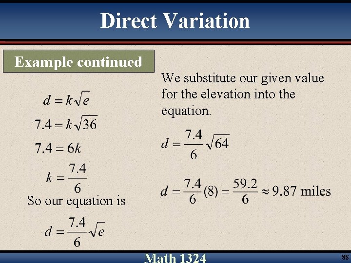
Direct Variation Example At sea, the distance to the horizon is directly proportional to the square root of the elevation of the observer. If a person who is 36 feet above water can see 7. 4 miles, find how far a person 64 feet above the water can see. Round your answer to two decimal places. Continued. 87

Direct Variation Example continued We substitute our given value for the elevation into the equation. So our equation is 88

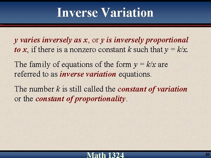
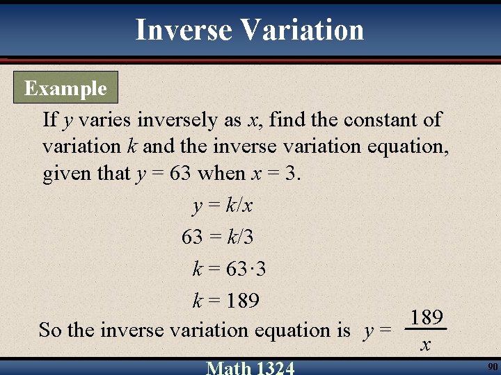
Inverse Variation y varies inversely as x, or y is inversely proportional to x, if there is a nonzero constant k such that y = k/x. The family of equations of the form y = k/x are referred to as inverse variation equations. The number k is still called the constant of variation or the constant of proportionality. 89

Inverse Variation Example If y varies inversely as x, find the constant of variation k and the inverse variation equation, given that y = 63 when x = 3. y = k/x 63 = k/3 k = 63· 3 k = 189 So the inverse variation equation is y = x 90

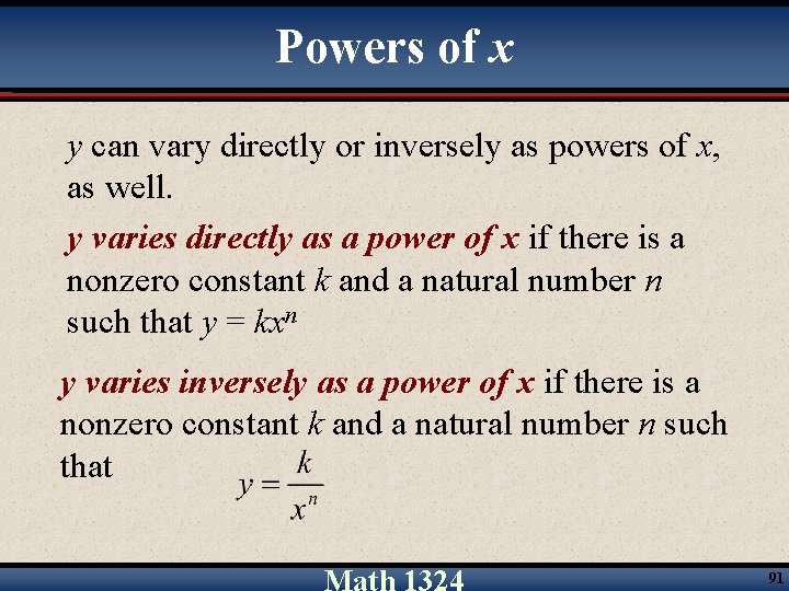
Powers of x y can vary directly or inversely as powers of x, as well. y varies directly as a power of x if there is a nonzero constant k and a natural number n such that y = kxn y varies inversely as a power of x if there is a nonzero constant k and a natural number n such that 91

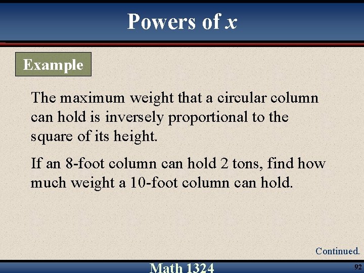
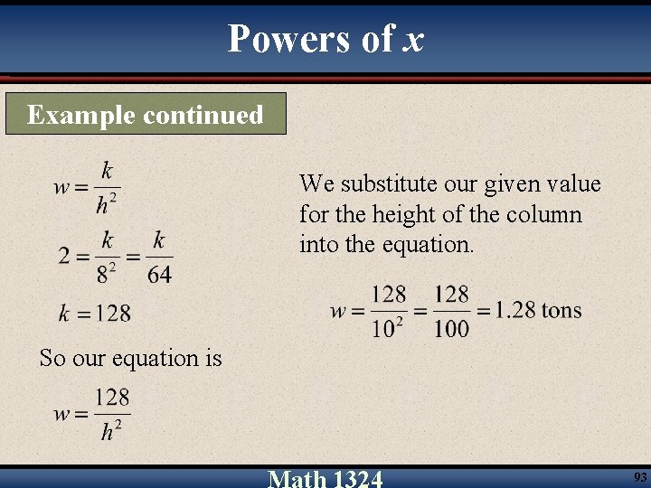
Powers of x Example The maximum weight that a circular column can hold is inversely proportional to the square of its height. If an 8 -foot column can hold 2 tons, find how much weight a 10 -foot column can hold. Continued. 92

Powers of x Example continued We substitute our given value for the height of the column into the equation. So our equation is 93