Chapter 2 DivideandConquer algorithms Divideandconquer Break up problem
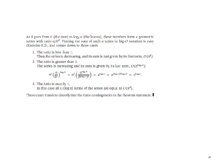
Chapter 2 Divide-and-Conquer algorithms Divide-and-conquer. Break up problem into several parts. Solve each part recursively. Combine solutions to sub-problems into overall solution. n n n Most common usage. Break up problem of size n into two equal parts of size ½n. Solve two parts recursively. Combine two solutions into overall solution in linear time. n n n Consequence. Brute force: n 2. Divide-and-conquer: n log n. n n 1
Example 1 Integer Multiplication
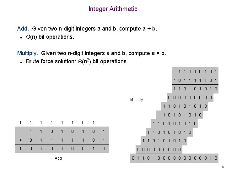
Integer Arithmetic Add. Given two n-digit integers a and b, compute a + b. O(n) bit operations. n Multiply. Given two n-digit integers a and b, compute a × b. Brute force solution: (n 2) bit operations. n 1 1 0 1 0 1 * 0 1 1 1 0 1 0 Multiply 0 0 0 0 0 1 1 0 1 0 1 1 1 0 1 0 1 + 0 1 1 1 0 1 0 1 0 Add 1 1 0 1 0 1 1 0 1 0 0 0 0 0 0 1 0 3
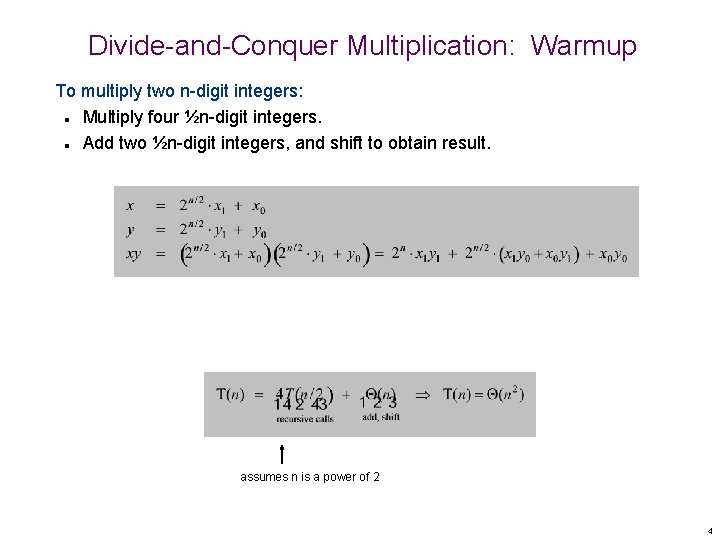
Divide-and-Conquer Multiplication: Warmup To multiply two n-digit integers: Multiply four ½n-digit integers. Add two ½n-digit integers, and shift to obtain result. n n assumes n is a power of 2 4
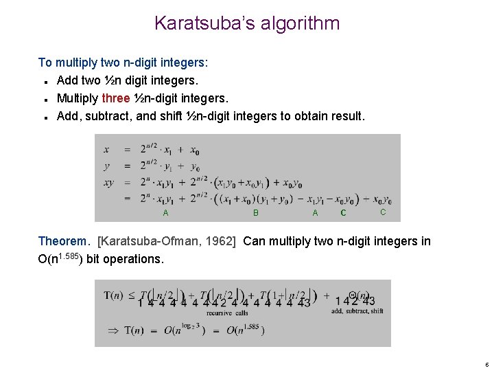
Karatsuba’s algorithm To multiply two n-digit integers: Add two ½n digit integers. Multiply three ½n-digit integers. Add, subtract, and shift ½n-digit integers to obtain result. n n n A B A C C Theorem. [Karatsuba-Ofman, 1962] Can multiply two n-digit integers in O(n 1. 585) bit operations. 5
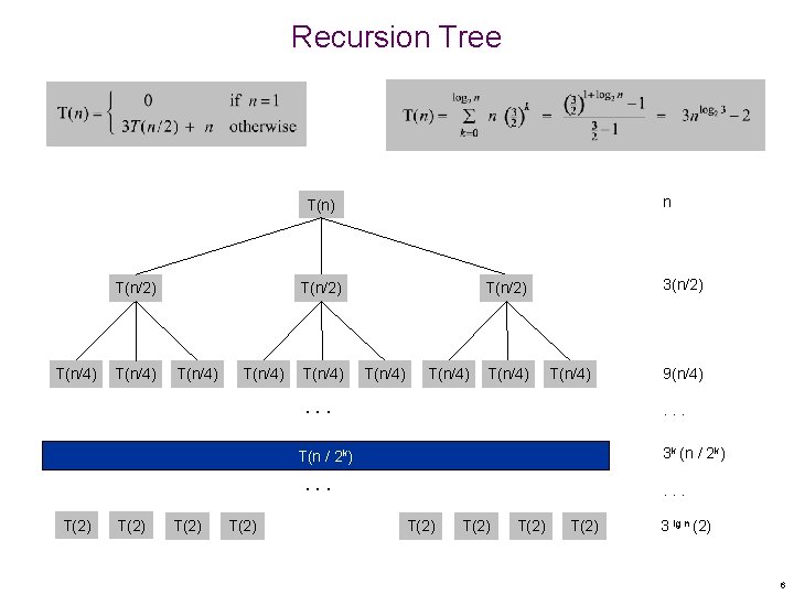
Recursion Tree n T(n) T(n/2) T(n/4) T(n/4) 3(n/2) T(n/4) T(n/4) . . . 3 k (n / 2 k) T(n / 2 k) . . . T(2) 9(n/4) . . . T(2) 3 lg n (2) 6
Example 2: Mergesort
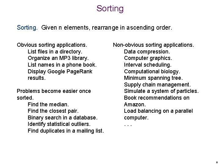
Sorting. Given n elements, rearrange in ascending order. Obvious sorting applications. List files in a directory. Organize an MP 3 library. List names in a phone book. Display Google Page. Rank results. Problems become easier once sorted. Find the median. Find the closest pair. Binary search in a database. Identify statistical outliers. Find duplicates in a mailing list. Non-obvious sorting applications. Data compression. Computer graphics. Interval scheduling. Computational biology. Minimum spanning tree. Supply chain management. Simulate a system of particles. Book recommendations on Amazon. Load balancing on a parallel computer. . 8
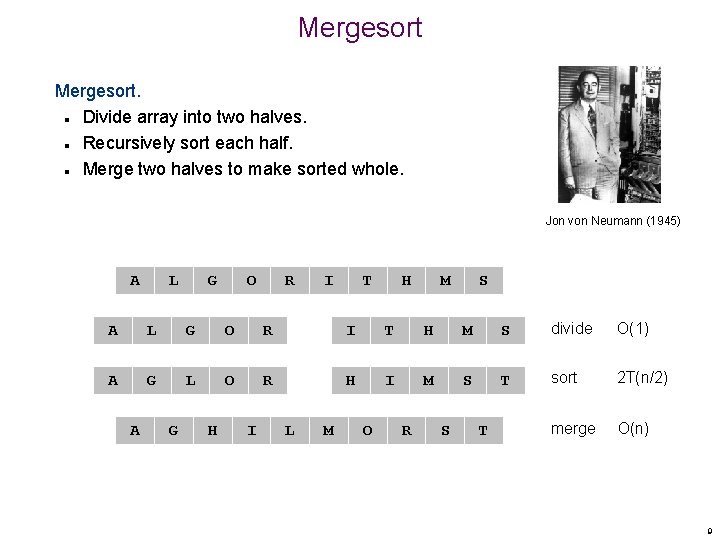
Mergesort. Divide array into two halves. Recursively sort each half. Merge two halves to make sorted whole. n n n Jon von Neumann (1945) A L G O R I T H M S divide O(1) A G L O R H I M S T sort 2 T(n/2) merge O(n) A G H I L M O R S T 9
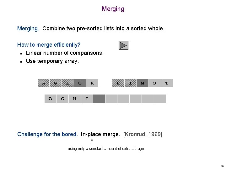
Merging. Combine two pre-sorted lists into a sorted whole. How to merge efficiently? Linear number of comparisons. Use temporary array. n n A G A L G O H R H I M S T I Challenge for the bored. In-place merge. [Kronrud, 1969] using only a constant amount of extra storage 10
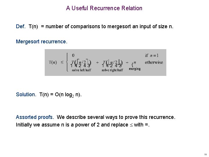
A Useful Recurrence Relation Def. T(n) = number of comparisons to mergesort an input of size n. Mergesort recurrence. Solution. T(n) = O(n log 2 n). Assorted proofs. We describe several ways to prove this recurrence. Initially we assume n is a power of 2 and replace with =. 11
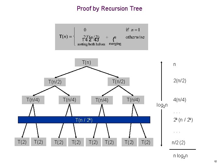
Proof by Recursion Tree T(n) n T(n/4) 2(n/2) T(n/2) T(n/4) log 2 n 4(n/4). . . 2 k (n / 2 k) T(n / 2 k) . . . T(2) T(2) n/2 (2) n log 2 n 12
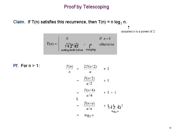
Proof by Telescoping Claim. If T(n) satisfies this recurrence, then T(n) = n log 2 n. assumes n is a power of 2 Pf. For n > 1: 13
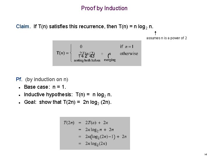
Proof by Induction Claim. If T(n) satisfies this recurrence, then T(n) = n log 2 n. assumes n is a power of 2 Pf. (by induction on n) Base case: n = 1. Inductive hypothesis: T(n) = n log 2 n. Goal: show that T(2 n) = 2 n log 2 (2 n). n n n 14
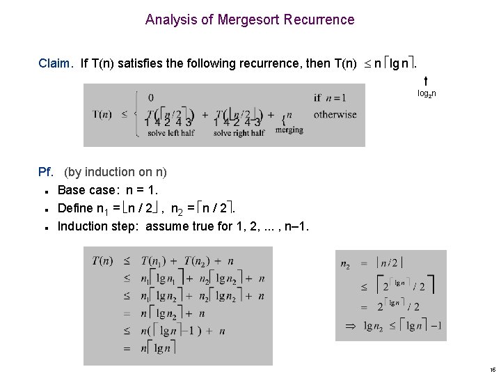
Analysis of Mergesort Recurrence Claim. If T(n) satisfies the following recurrence, then T(n) n lg n. log 2 n Pf. (by induction on n) Base case: n = 1. Define n 1 = n / 2 , n 2 = n / 2. Induction step: assume true for 1, 2, . . . , n– 1. n n n 15
16
17
18
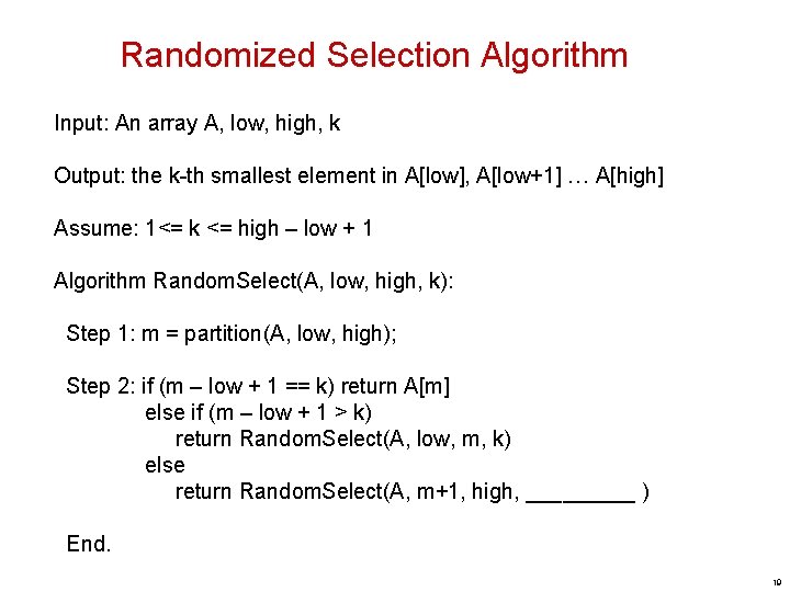
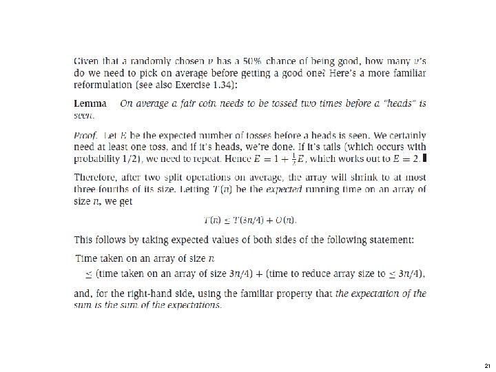
Randomized Selection Algorithm Input: An array A, low, high, k Output: the k-th smallest element in A[low], A[low+1] … A[high] Assume: 1<= k <= high – low + 1 Algorithm Random. Select(A, low, high, k): Step 1: m = partition(A, low, high); Step 2: if (m – low + 1 == k) return A[m] else if (m – low + 1 > k) return Random. Select(A, low, m, k) else return Random. Select(A, m+1, high, _____ ) End. 19
20
21
The Fast Fourier Transform FFT 22
Outline and Reading Polynomial Multiplication Problem • Primitive Roots of Unity (page 63) • The FFT Algorithm (page 64) • Integer Multiplication ([AHU] Section 8. 1) • Java FFT Integer Multiplication • FFT 23
Polynomials Polynomial: In general, FFT 24
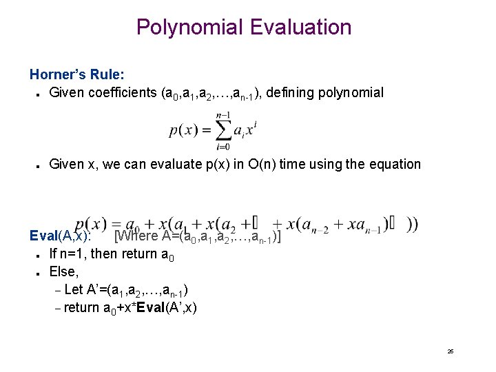
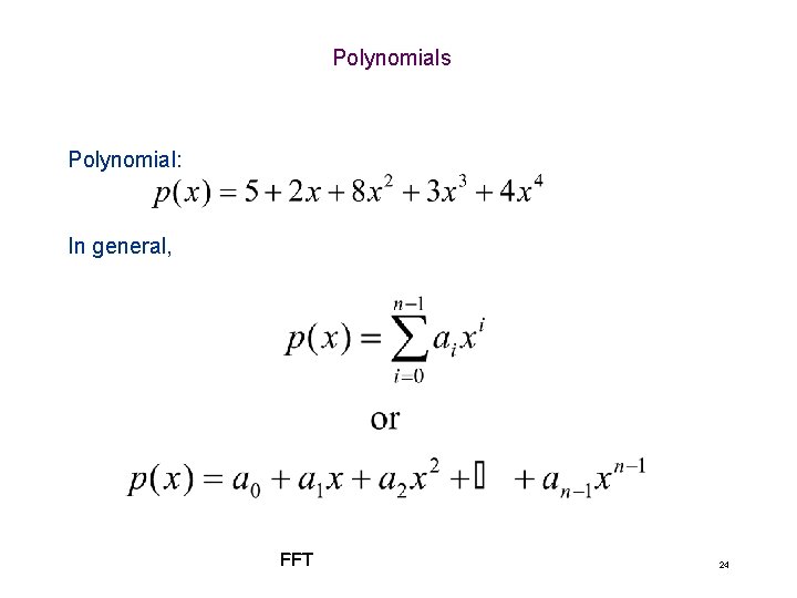
Polynomial Evaluation Horner’s Rule: Given coefficients (a 0, a 1, a 2, …, an-1), defining polynomial n n Given x, we can evaluate p(x) in O(n) time using the equation Eval(A, x): [Where A=(a 0, a 1, a 2, …, an-1)] If n=1, then return a 0 Else, – Let A’=(a 1, a 2, …, an-1) – return a 0+x*Eval(A’, x) n n 25
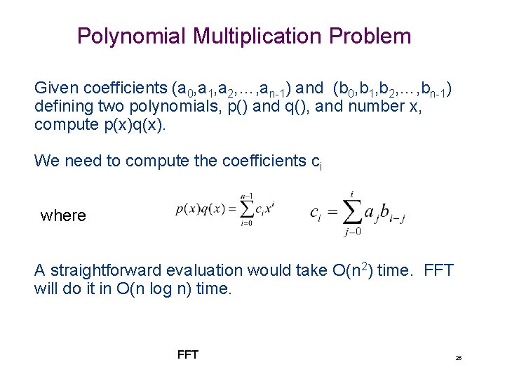
Polynomial Multiplication Problem Given coefficients (a 0, a 1, a 2, …, an-1) and (b 0, b 1, b 2, …, bn-1) defining two polynomials, p() and q(), and number x, compute p(x)q(x). We need to compute the coefficients ci where A straightforward evaluation would take O(n 2) time. FFT will do it in O(n log n) time. FFT 26
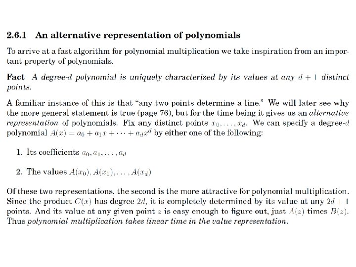
Polynomial Interpolation & Polynomial Multiplication Given a set of n points in the plane with distinct x-coordinates, there is exactly one (n-1)-degree polynomial going through all these points. Alternate approach to computing p(x)q(x): n n n Calculate p() on 2 n x-values, x 0, x 1, …, x 2 n-1. Calculate q() on the same 2 n x values. Find the (2 n-1)-degree polynomial that goes through the points {(x 0, p(x 0)q(x 0)), (x 1, p(x 1)q(x 1)), …, (x 2 n-1, p(x 2 n-1)q(x 2 n-1))}. Unfortunately, a straightforward evaluation would still take O(n 2) time, as we would need to apply an O(n)-time Horner’s Rule evaluation to 2 n different points. FFT will do it in O(n log n) time, by picking 2 n points that are easy to evaluate… FFT 27
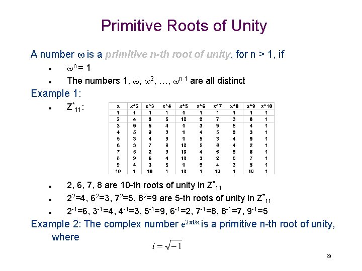
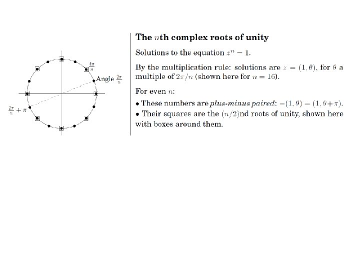
Primitive Roots of Unity A number w is a primitive n-th root of unity, for n > 1, if n n wn = 1 The numbers 1, w, w 2, …, wn-1 are all distinct Example 1: n n Z*11: 2, 6, 7, 8 are 10 -th roots of unity in Z*11 22=4, 62=3, 72=5, 82=9 are 5 -th roots of unity in Z*11 2 -1=6, 3 -1=4, 4 -1=3, 5 -1=9, 6 -1=2, 7 -1=8, 8 -1=7, 9 -1=5 Example 2: The complex number e 2 pi/n is a primitive n-th root of unity, where 28
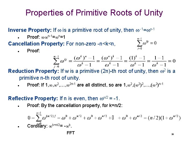
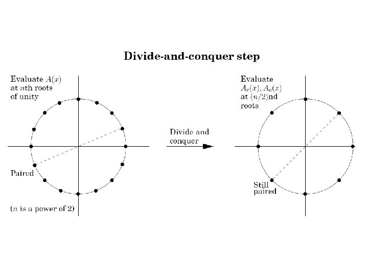
Properties of Primitive Roots of Unity Inverse Property: If w is a primitive root of unity, then w -1=wn-1 n Proof: wwn-1=wn=1 Cancellation Property: For non-zero -n<k<n, n Proof: Reduction Property: If w is a primitive (2 n)-th root of unity, then w 2 is a primitive n-th root of unity. n Proof: If 1, w, w 2, …, w 2 n-1 are all distinct, so are 1, w 2, (w 2)2, …, (w 2)n-1 Reflective Property: If n is even, then wn/2 = -1. n Proof: By the cancellation property, for k=n/2: n Corollary: wk+n/2= -wk. FFT 29
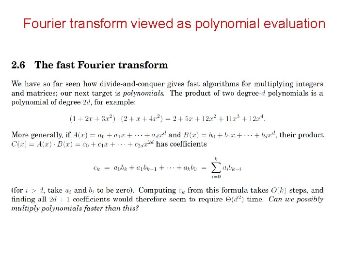
Fourier transform viewed as polynomial evaluation
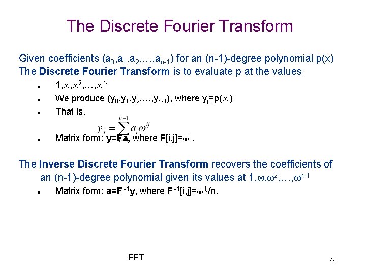
The Discrete Fourier Transform Given coefficients (a 0, a 1, a 2, …, an-1) for an (n-1)-degree polynomial p(x) The Discrete Fourier Transform is to evaluate p at the values n 1, w, w 2, …, wn-1 We produce (y 0, y 1, y 2, …, yn-1), where yj=p(wj) That is, n Matrix form: y=Fa, where F[i, j]=wij. n n The Inverse Discrete Fourier Transform recovers the coefficients of an (n-1)-degree polynomial given its values at 1, w, w 2, …, wn-1 n Matrix form: a=F -1 y, where F -1[i, j]=w-ij/n. FFT 34
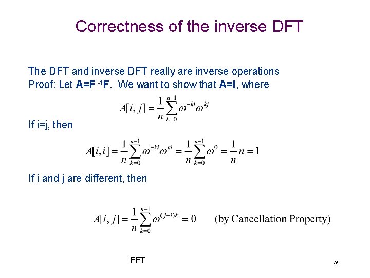
Correctness of the inverse DFT The DFT and inverse DFT really are inverse operations Proof: Let A=F -1 F. We want to show that A=I, where If i=j, then If i and j are different, then FFT 35
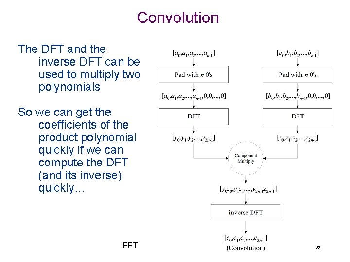
Convolution The DFT and the inverse DFT can be used to multiply two polynomials So we can get the coefficients of the product polynomial quickly if we can compute the DFT (and its inverse) quickly… FFT 36
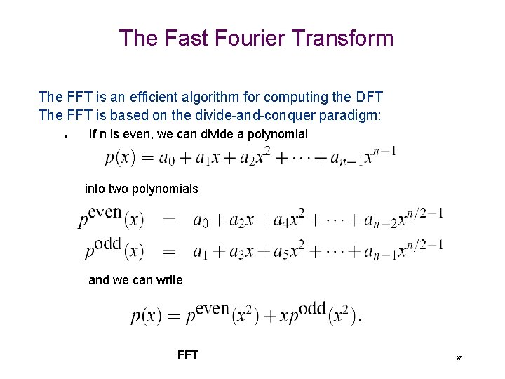
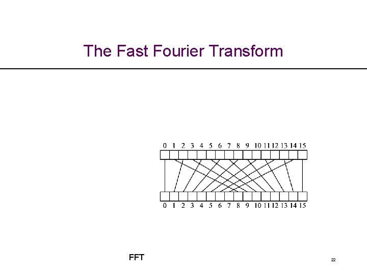
The Fast Fourier Transform The FFT is an efficient algorithm for computing the DFT The FFT is based on the divide-and-conquer paradigm: n If n is even, we can divide a polynomial into two polynomials and we can write FFT 37
![The FFT Algorithm The running time is O(n log n). [inverse FFT is similar] The FFT Algorithm The running time is O(n log n). [inverse FFT is similar]](http://slidetodoc.com/presentation_image/793fab253c4b555efdb9faebdeae7032/image-38.jpg)
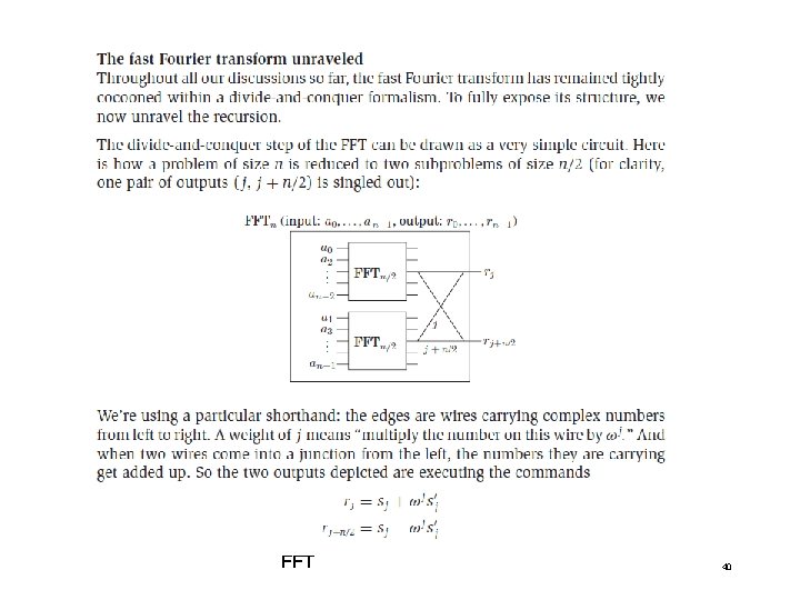
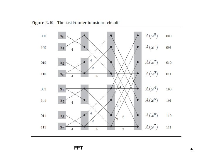
The FFT Algorithm The running time is O(n log n). [inverse FFT is similar] FFT 38
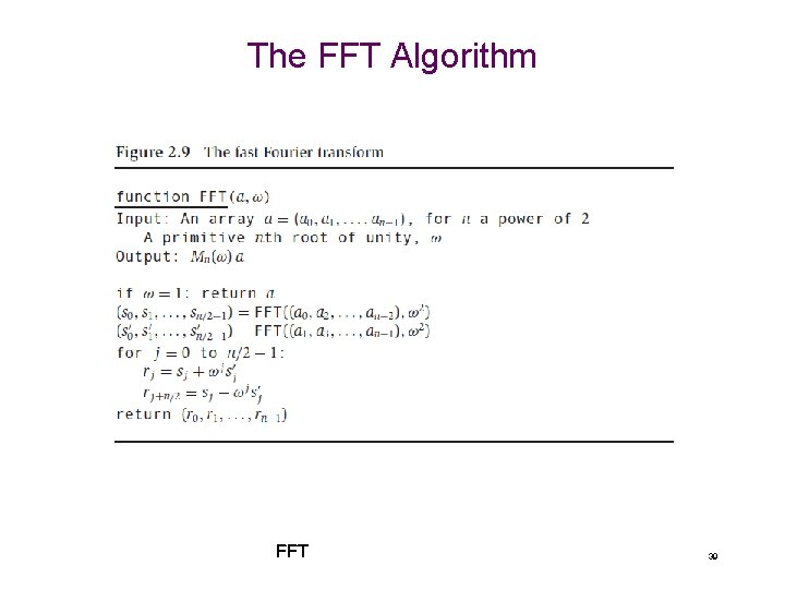
The FFT Algorithm FFT 39
FFT 40
FFT 41
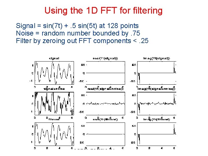
Using the 1 D FFT for filtering Signal = sin(7 t) +. 5 sin(5 t) at 128 points Noise = random number bounded by. 75 Filter by zeroing out FFT components <. 25 CS 267 Lecture 21
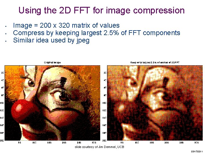
Using the 2 D FFT for image compression • • • Image = 200 x 320 matrix of values Compress by keeping largest 2. 5% of FFT components Similar idea used by jpeg slide courtesy of Jim Demmel, UCB 03/17/2011
- Slides: 43