Chapter 2 Discretetime signals and systems Content and

Chapter 2: Discrete-time signals and systems Content and Figures are from Discrete-Time Signal Processing, 2 e by Oppenheim, Shafer and Buck, © 1999 -2000 Prentice Hall Inc.

2. 0 DSP: applications • Speech, audio – Noise reduction (Dolby), compression (MP 3), … • Radar – filtering, movement detection, … • Image processing – Compression, pattern recognition, segmentation, … • Biomedical – Monitoring, analysis, tele-medicine, … Chapter 2: Discrete time signals and systems 1

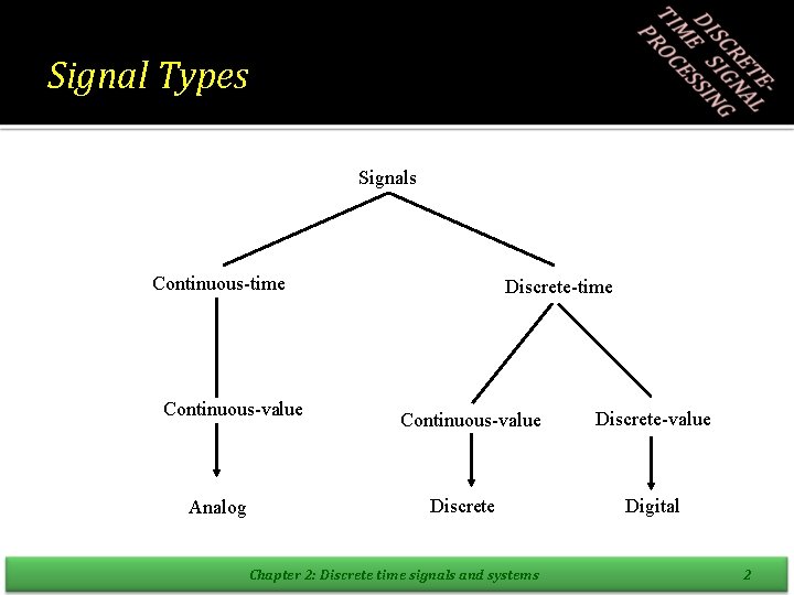
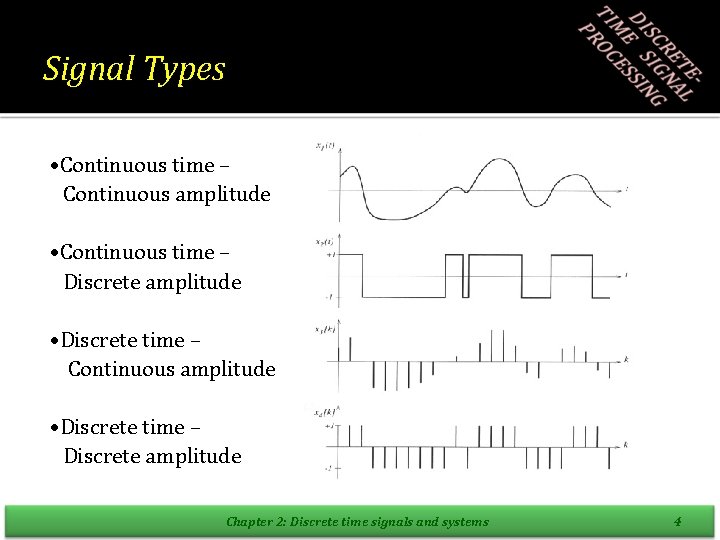
Signal Types Signals Continuous-time Continuous-value Analog Discrete-time Continuous-value Discrete Chapter 2: Discrete time signals and systems Discrete-value Digital 2

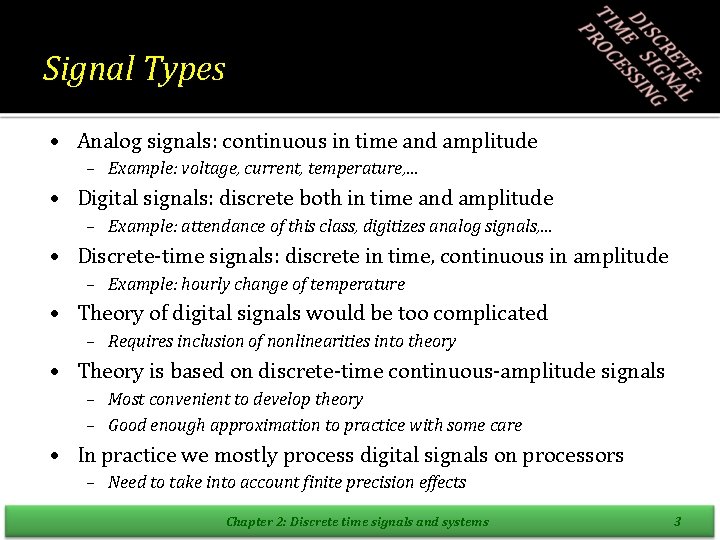
Signal Types • Analog signals: continuous in time and amplitude – Example: voltage, current, temperature, … • Digital signals: discrete both in time and amplitude – Example: attendance of this class, digitizes analog signals, … • Discrete-time signals: discrete in time, continuous in amplitude – Example: hourly change of temperature • Theory of digital signals would be too complicated – Requires inclusion of nonlinearities into theory • Theory is based on discrete-time continuous-amplitude signals – Most convenient to develop theory – Good enough approximation to practice with some care • In practice we mostly process digital signals on processors – Need to take into account finite precision effects Chapter 2: Discrete time signals and systems 3

Signal Types • Continuous time – Continuous amplitude • Continuous time – Discrete amplitude • Discrete time – Continuous amplitude • Discrete time – Discrete amplitude Chapter 2: Discrete time signals and systems 4

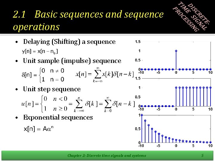
2. 1 Basic sequences and sequence operations • Delaying (Shifting) a sequence • Unit sample (impulse) sequence • Unit step sequence • Exponential sequences Chapter 2: Discrete time signals and systems 5

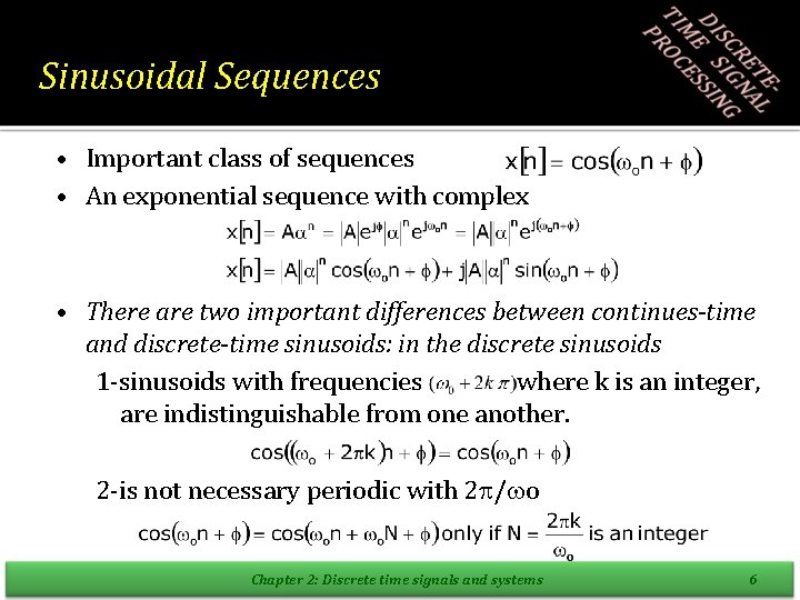
Sinusoidal Sequences • Important class of sequences • An exponential sequence with complex • There are two important differences between continues-time and discrete-time sinusoids: in the discrete sinusoids 1 -sinusoids with frequencies where k is an integer, are indistinguishable from one another. 2 -is not necessary periodic with 2 / o Chapter 2: Discrete time signals and systems 6

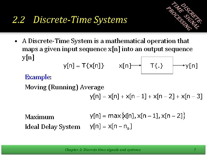
2. 2 Discrete-Time Systems • A Discrete-Time System is a mathematical operation that maps a given input sequence x[n] into an output sequence y[n] Example: Moving (Running) Average Maximum Ideal Delay System Chapter 2: Discrete time signals and systems 7

Memoryless System A system is memoryless if the output y[n] at every value of n depends only on the input x[n] at the same value of n Example : Square Sign counter example: Ideal Delay System Chapter 2: Discrete time signals and systems 8

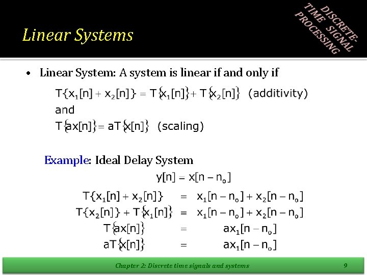
Linear Systems • Linear System: A system is linear if and only if Example: Ideal Delay System Chapter 2: Discrete time signals and systems 9

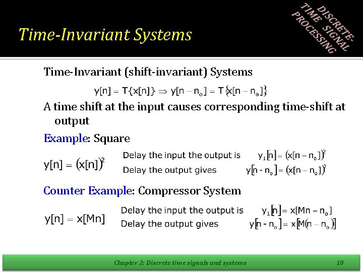
Time-Invariant Systems Time-Invariant (shift-invariant) Systems A time shift at the input causes corresponding time-shift at output Example: Square Counter Example: Compressor System Chapter 2: Discrete time signals and systems 10

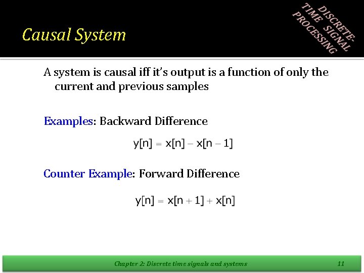
Causal System A system is causal iff it’s output is a function of only the current and previous samples Examples: Backward Difference Counter Example: Forward Difference Chapter 2: Discrete time signals and systems 11

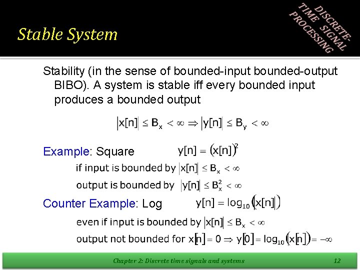
Stable System Stability (in the sense of bounded-input bounded-output BIBO). A system is stable iff every bounded input produces a bounded output Example: Square Counter Example: Log Chapter 2: Discrete time signals and systems 12

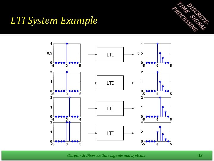
LTI System Example Chapter 2: Discrete time signals and systems 13

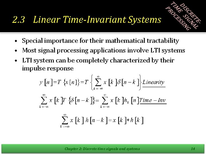
2. 3 Linear Time-Invariant Systems • Special importance for their mathematical tractability • Most signal processing applications involve LTI systems • LTI system can be completely characterized by their impulse response Chapter 2: Discrete time signals and systems 14

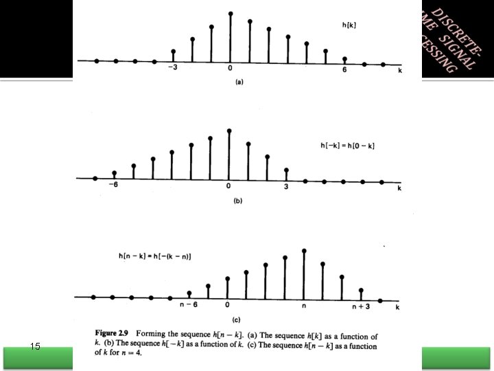
15 Digital Signal Processing

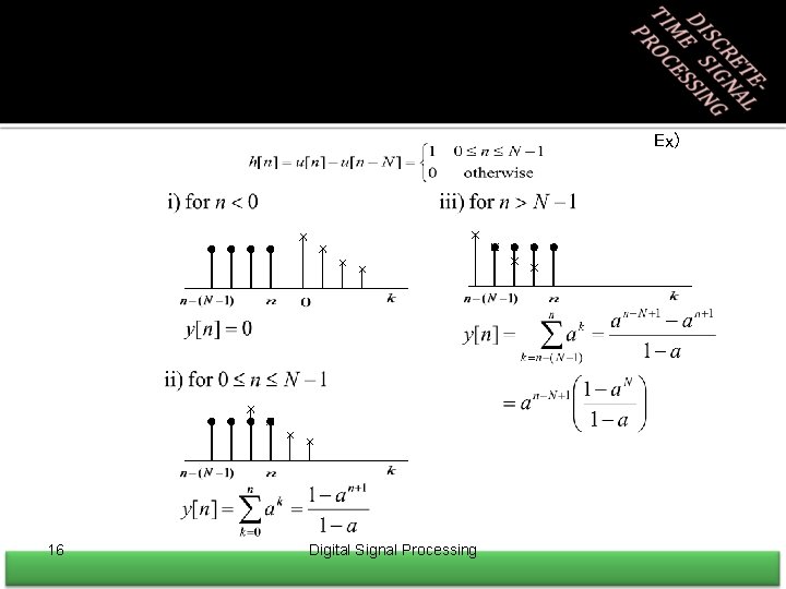
Ex) 16 Digital Signal Processing

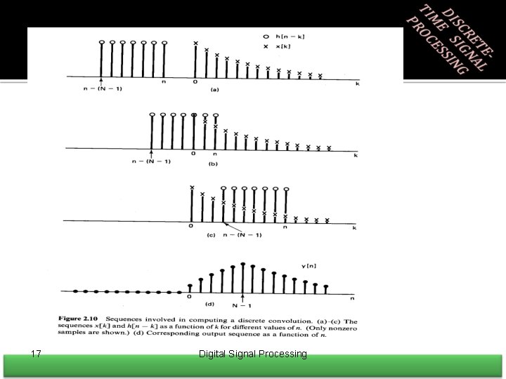
17 Digital Signal Processing

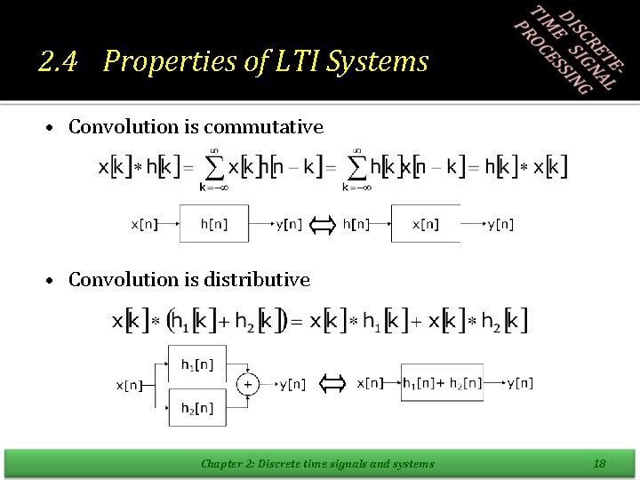
2. 4 Properties of LTI Systems • Convolution is commutative • Convolution is distributive Chapter 2: Discrete time signals and systems 18

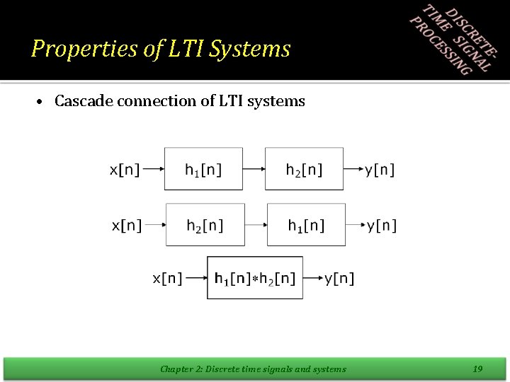
Properties of LTI Systems • Cascade connection of LTI systems Chapter 2: Discrete time signals and systems 19

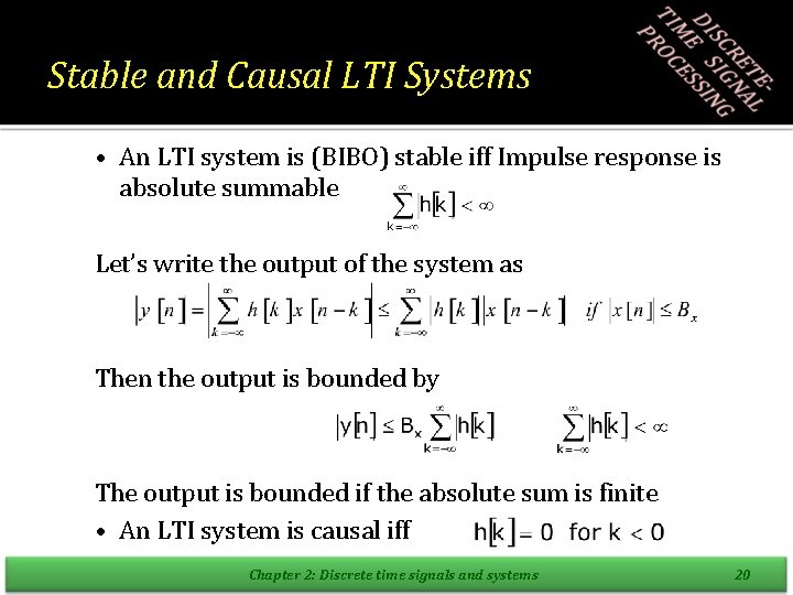
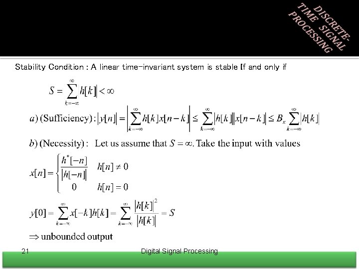
Stable and Causal LTI Systems • An LTI system is (BIBO) stable iff Impulse response is absolute summable Let’s write the output of the system as Then the output is bounded by The output is bounded if the absolute sum is finite • An LTI system is causal iff Chapter 2: Discrete time signals and systems 20

Stability Condition : A linear time-invariant system is stable If and only if 21 Digital Signal Processing

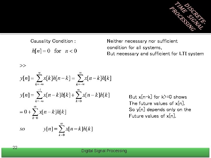
Causality Condition : Neither necessary nor sufficient condition for all systems, But necessary and sufficient for LTI system But x[n-k] for k>=0 shows The future values of x[n]. So y[n] depends only on the Future values of x[n]. 22 Digital Signal Processing

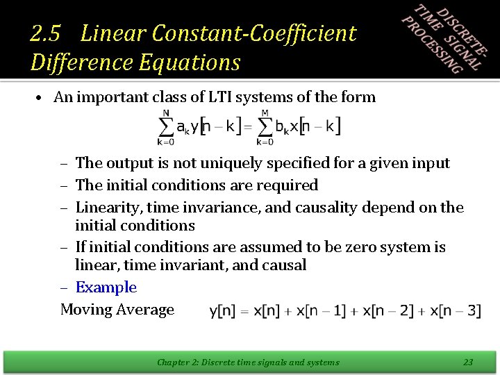
2. 5 Linear Constant-Coefficient Difference Equations • An important class of LTI systems of the form – The output is not uniquely specified for a given input – The initial conditions are required – Linearity, time invariance, and causality depend on the initial conditions – If initial conditions are assumed to be zero system is linear, time invariant, and causal – Example Moving Average Chapter 2: Discrete time signals and systems 23

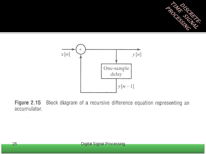
• Linear Constant-Coefficient Difference Equations Ex) X[n] is the difference of y[n] 24 Digital Signal Processing

25 Digital Signal Processing

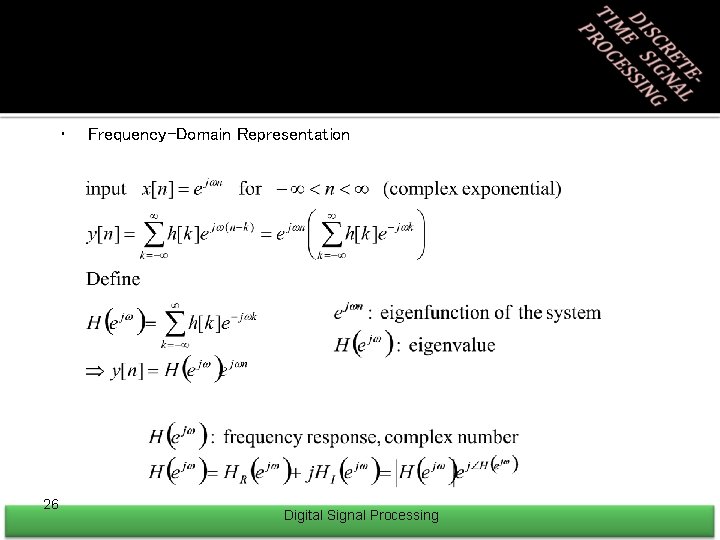
• 26 Frequency-Domain Representation Digital Signal Processing

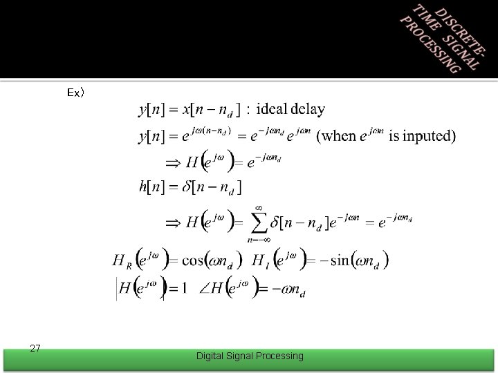
Ex) 27 Digital Signal Processing

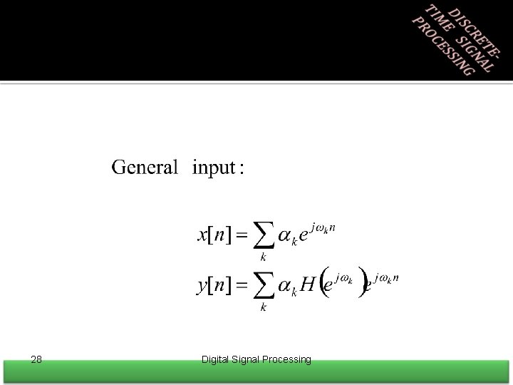
28 Digital Signal Processing

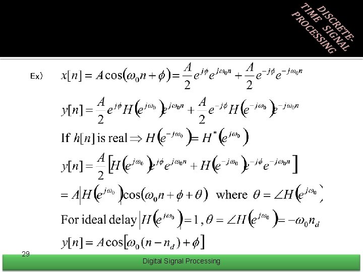
Ex) 29 Digital Signal Processing

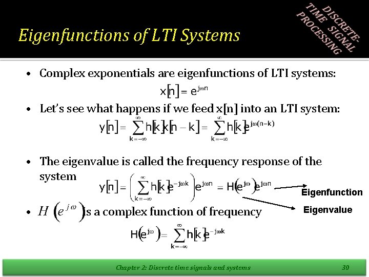
Eigenfunctions of LTI Systems • Complex exponentials are eigenfunctions of LTI systems: • Let’s see what happens if we feed x[n] into an LTI system: • The eigenvalue is called the frequency response of the system Eigenfunction • is a complex function of frequency Chapter 2: Discrete time signals and systems Eigenvalue 30

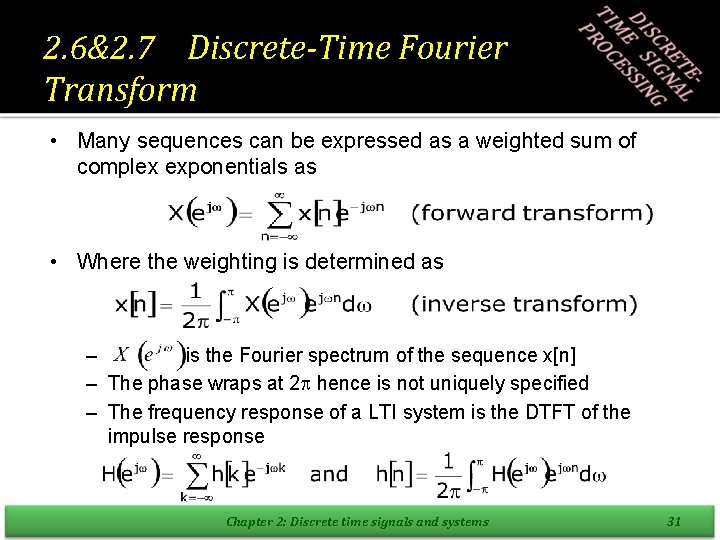
2. 6&2. 7 Discrete-Time Fourier Transform • Many sequences can be expressed as a weighted sum of complex exponentials as • Where the weighting is determined as – is the Fourier spectrum of the sequence x[n] – The phase wraps at 2 hence is not uniquely specified – The frequency response of a LTI system is the DTFT of the impulse response Chapter 2: Discrete time signals and systems 31

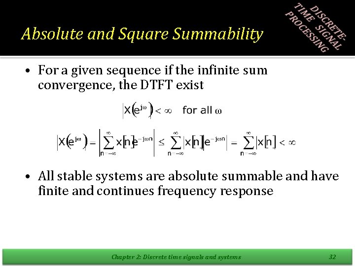
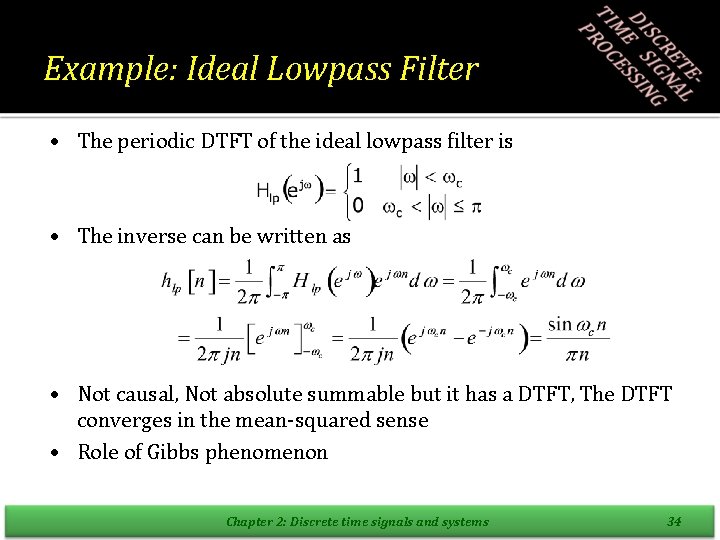
Absolute and Square Summability • For a given sequence if the infinite sum convergence, the DTFT exist • All stable systems are absolute summable and have finite and continues frequency response Chapter 2: Discrete time signals and systems 32

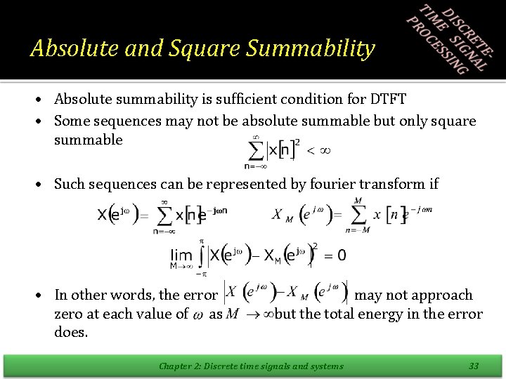
Absolute and Square Summability • Absolute summability is sufficient condition for DTFT • Some sequences may not be absolute summable but only square summable • Such sequences can be represented by fourier transform if • In other words, the error zero at each value of as does. may not approach but the total energy in the error Chapter 2: Discrete time signals and systems 33

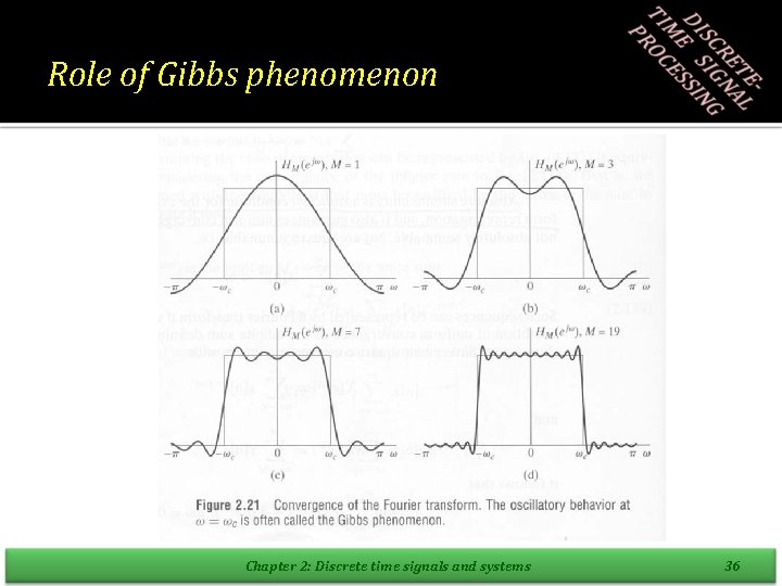
Example: Ideal Lowpass Filter • The periodic DTFT of the ideal lowpass filter is • The inverse can be written as • Not causal, Not absolute summable but it has a DTFT, The DTFT converges in the mean-squared sense • Role of Gibbs phenomenon Chapter 2: Discrete time signals and systems 34

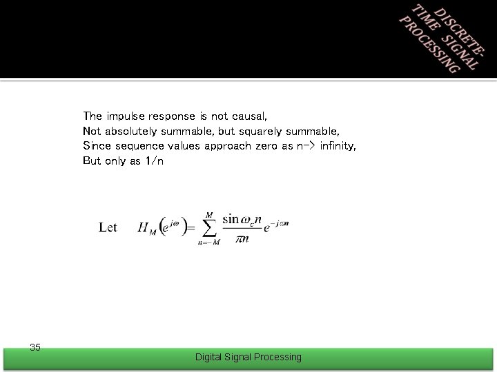
Ex) The impulse response is not causal, Not absolutely summable, but squarely summable, Since sequence values approach zero as n-> infinity, But only as 1/n 35 Digital Signal Processing

Role of Gibbs phenomenon Chapter 2: Discrete time signals and systems 36

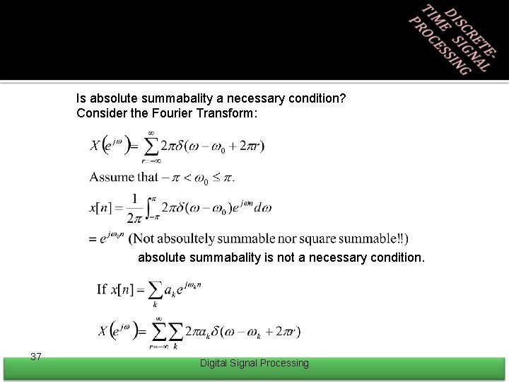
Is absolute summabality a necessary condition? Consider the Fourier Transform: absolute summabality is not a necessary condition. 37 Digital Signal Processing

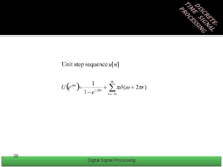
38 Digital Signal Processing

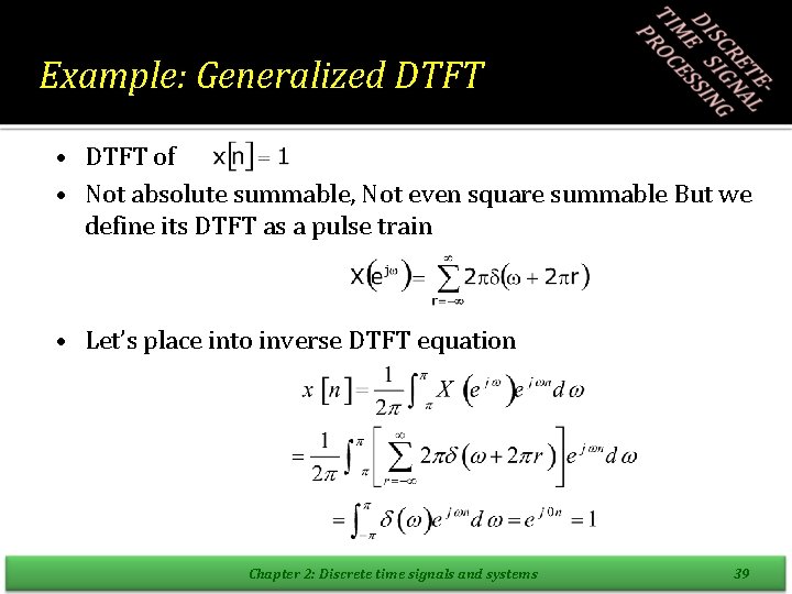
Example: Generalized DTFT • DTFT of • Not absolute summable, Not even square summable But we define its DTFT as a pulse train • Let’s place into inverse DTFT equation Chapter 2: Discrete time signals and systems 39

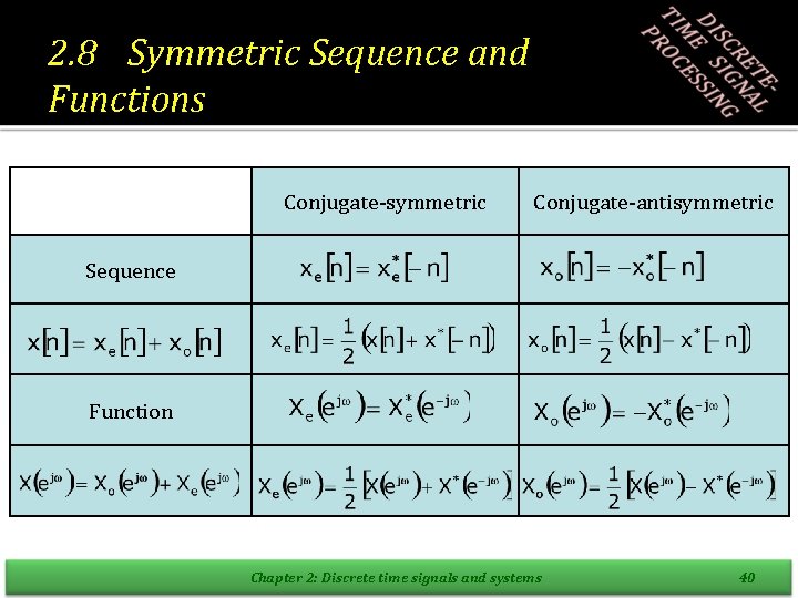
2. 8 Symmetric Sequence and Functions Conjugate-symmetric Conjugate-antisymmetric Sequence Function Chapter 2: Discrete time signals and systems 40

Properties of DTFT Sequence x[n] Discrete-Time Fourier Transform X(ej ) x*[n] X*(e-j ) x*[-n] X*(ej ) Re{x[n]} Xe(ej ) (conjugate-symmetric part) j. Im{x[n]} Xo(ej ) (conjugate-antisymmetric part) xe[n] XR(ej )= Re{X(ej )} xo[n] j. XI(ej )= j. Im{X(ej )} Any real x[n] X(ej )=X*(e-j ) (conjugate symmetric) Any real x[n] XR(ej )=XR(e-j ) (real part is even) Any real x[n] XI(ej )=-XI(e-j ) (imaginary part is odd) Any real x[n] |X(ej )|=|X(e-j )| (magnitude is even) Any real x[n] X(ej )=- X(e-j ) (phase is odd) xe[n] XR(ej ) xo[n] j. XI(ej ) Chapter 2: Discrete time signals and systems 41

Example: Illustration of Symmetry Properties • DTFT of the real sequence x[n]=anu[n] • Some properties are Chapter 2: Discrete time signals and systems 42

2. 9 Fourier Transform Theorems x[n] y[n] X(ej ) Y(ej ) ax[n]+by[n] a. X(ej )+b. Y(ej ) x[n-nd] x[-n] X(e-j ) nx[n] y[n] X(ej )Y(ej ) x[n]y[n] Chapter 2: Discrete time signals and systems 43

Fourier Transform Pairs Sequence DTFT [n-no] u[n] cos( on+ ) Chapter 2: Discrete time signals and systems 44

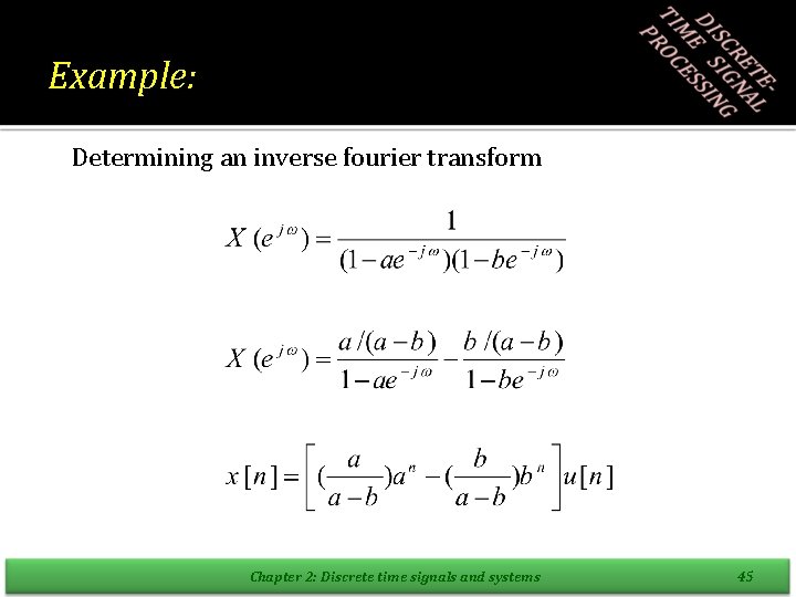
Example: Determining an inverse fourier transform Chapter 2: Discrete time signals and systems 45

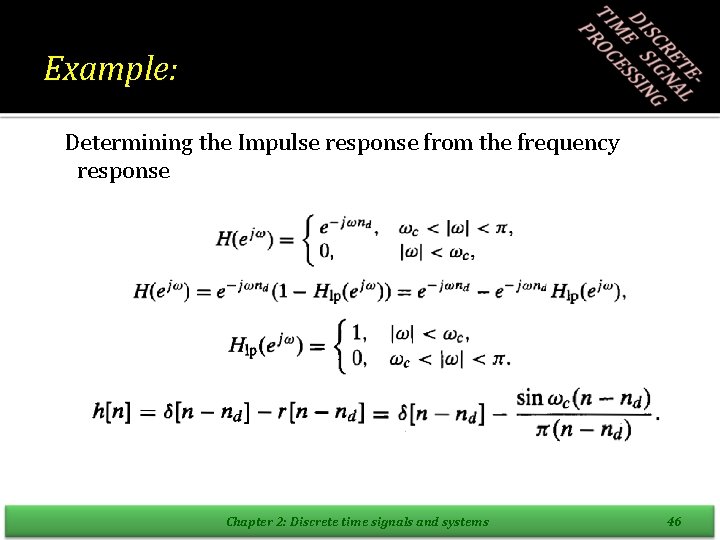
Example: Determining the Impulse response from the frequency response Chapter 2: Discrete time signals and systems 46

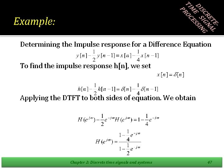
Example: Determining the Impulse response for a Difference Equation To find the impulse response h[n], we set Applying the DTFT to both sides of equation. We obtain Chapter 2: Discrete time signals and systems 47

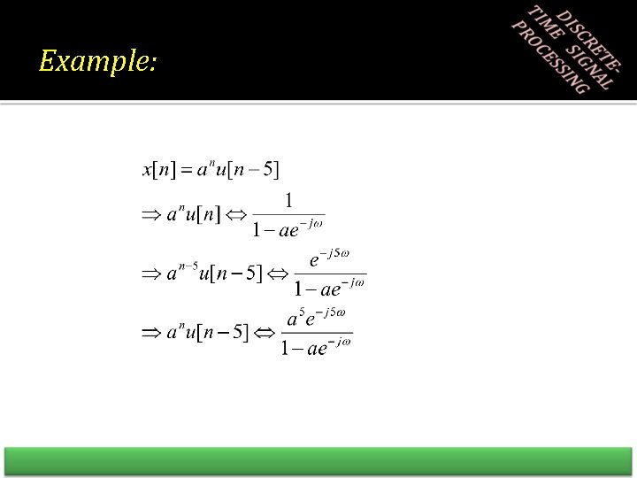
Example: