Chapter 2 Digital Image Fundamentals 2 1 Human

Chapter 2 Digital Image Fundamentals

2. 1 Human Visual System Purpose of study : Improvement of images for use by a human observer (1) Physical Structure of the Eye Cornea : convex lens, refracting the rays Aqueous humor Iris : a variable aperture to control the amount of light

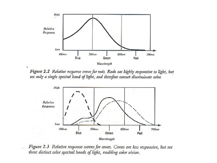
Lens : Controls the focal length to focus at retina Vitreous humor Retina : Composed of photoreceptors to convert the intensity and color of light to neural signals ( 108 elements) Types of photo Receptors Rods : to respond to broad-spectrum color light for lowlight vision, and therefore cannot discriminate color. Cones : for day-light vision. Three different types of cones for color vision (trichromacy)

Distribution of rods and cones - Color perception is best for the objects that we are viewing directly forward -Relative insensitivity of cones also accounts for our inability to perceive color under low-light conditions

Optic nerve and visual cortex lights Rods/Cones neural impulses Optic Nerve Visual Cortex Processing (brain) 2. 2 Image Processing in the Eye Weber’s law decision

-The difference in perceived brightness of the steps does not Appear equal -The eye cannot see the same intensity increments in the bright regions that it sees in the dark regions

Note) In DIP, simple darkening of bright regions can make undetectably minute intensity changes perceptible Lateral Inhibitions Simultaneous Contrast The square in the left side is brighter than that in the right side

② Match band effect Visual system accentuates sharp intensity changes Human eye is sensitive to the changes of intensities (edges) Note : Second–Order System Frequency Response of HVS

Size of image : M x M fmax = M/2/ = M/2 (Cycles / degree) = 2 tan-1(0. 5 x/6 H) (degree)

Sensitivity curve Other Properties of HVS : Digital Picture Processing, volume 1, Chapter 3, Azriel Rosenfeld and Avinash C. kak

2. 3 Sampling and Quantization Uniform sampling and quantization F(x, y) = f(0, 0) f(0, 1) …………… f(0, M-1) f(1, 0) f(1, 1) …………… f(1, M-1) f(N-1, 0) f(N-1, 1) …. . f(N-1, M-1) N x M Size of DI N = 2 n , M = 2 k Gray level G = 2 m # of bits = N x M x m

Effect of Image Resolution (a)1024 x 1024 (b) 512 x 512 (d) 128 x 128 (e) 64 x 64 (c) 256 x 256 (f) 32 x 32

Effect of Quantization Levels (a) 8 bit (e) 4 bit (b) 7 bit (c) 6 bit (f) 3 bit (g) 2 bit (d) 5 bit (h) 1 bit

Isopreference curves Figure 2. 12 Isopreference curves for (a) face (b) cameraman, and (c) crowd. (From Huang [1965] -The quality of the images tends to increase as N and m are increased Note : Exceptional Case For fixed N, the quality is improved by decreasing m. (contrast)

-The curves tend to become more vertical Note : For images with a large amount of detail only a few gray levels are needed -The curves depart markedly from the curves of constant b = N 2 m Non-uniform Sampling / Quantization - Fine sampling is the neighborhood of sharp gray-level transitions whereas coarse sampling in relatively smooth regions -Quantization according to the sensitivity of HVS. (Subband Coding)

2. 4 Some Basic Relationships Between Pixel Neighbor of a pixel N 4(p) ND(p) x x p x N 8(p) x x x p x x N 8(p) = N 4(p) ND(p)

Connectivity V = Set of gray- level values used to define connectivity - 4 -connectivity q q p and one of q V - 8 -connectivity q q q q p and one of q V

- m-connectivity ① q is in N 4(p) or ② q is in ND(p) and the set N 4(p) N 4(q) is empty - A pixel p is adjacent to a pixel q if they are connected - Path / length (x 0, y 0)(x 1, y 1)…(xn, yn)

- Connected If p and q pixels of an image subset S , then p is connected to q in S if there is a path from p to q consisting entire of pixels in S - Connected component S For any pixel p in S , the set of pixels in S that are connected to p

Labeling of Connected Components - With 4 -Connected Components : t r p If p = 0, move to next scanning position Otherwise (p=1), if r = t = 0, then assign a new label if , then assign the label that is equal to 1 if r = t = 1 , and they have the same label, then assign the label if r = t= 1 , and they have the different labels, then assign one of the labels and make a note they are equivalent merge the equivalent labels

- With 8 -connected components s r t p q If p=0 then move to next position If p=1 then If only one of neighbors is equal to 1 , then assign the label. If none of neighbors is equal to 1, then assign a new label. If two or more neighbor are equal to 1, and they have different labels, then assign are of then and make note that they are equivalent label. Merge the equivalent labels

Relations, Equivalence, and Transitive Closure - Binary Relation R on set A Ex. R = relation of 4 -connected Definitions : Equivalence Relations (a) reflexive if for each a ∈ A , a. Ra (b) symmetric if for each a and b ∈ A, a. Rb → b. Ra (c) transitive if for a, b, and c ∈ A, a. Rb and b. Rc → a. Rc Property : If R is an equivalence relation on a set A, then A can be divided into disjoint subsets, called equivalence classes.

Ex. Adjacent Matrix Note : reflexive relation symmetric relation every diagonal element = 1 symmetric matrix

- Transitive Closure of R : R+ Ex. Note : 1) b. Rd and d. Rb b. Rb d. Rb and b. Rd d. Rd 2) B+ = B + BBB + + (B)n multiplication AND addition OR

Distance Measures D is a distance function or metric if Ex) Euclidean Distance

length of the shortest path = distance in D 4 and D 8 length of path in m-connectivity not unique Ex) m-distance from p to p 4 = 2 or m-distance from p to p 4 = 3

Relations, Equivalence, and Transitive Closure - Binary Relation R on set A Ex.

Property : If R is an equivalence relation on a set A , then A can be divided into & disjoint subsets, called equivalence classes Ex. Note : reflexive relation symmetric relation every diagonal element = 1 symmetric matrix

- Transitive Closure of R : R+ Note : 1) 2) multiplication addition AND OR

Arithmetic and Logic Operations -pixel by pixel operation : p p +q –q *q /q Multiplication pixel p AND q p OR q Binary image Note : Quantization of Gray-level image <pixel wise>

Ex. Some Examples of Logic Operations on Binary Images

- neighborhood oriented operation : mask operation w 1 w 2 w 3 w 4 w 5 w 6 w 7 w 8 w 9 Computationally expensive operation 512 × 512 3 × 3 mask Multiplication 9 × 512 operation Addition 8 × 512 parallel operation is needed. - object oriented operation Note : The complexity and parallel architecture that depends on the operation look-up Table / SIMD / MIMD

Imaging Geometry Some basic Transform - Translation z Z y x Y X World coordinate system (X, Y, Z) V* = T · V

Note : Movement of object point in the same coordinate systems Ex. Change of coordinate systems for on object point Ex.

- Scaling By factors Sx, Sy, Sz along X, Y, Z axis - Rotation rotation about z-axis Z θ α θ X θ β Y

rotation about x-axis rotation about y-axis - Concatenation and inverse transform , where For m-points, m

- Inverse Transform Perspective Transform y, Y x, X (X, Y, Z) Image plane z, Z Lens center (x, y)

- Homogeneous coordinates

- Inverse perspective transform Note : It is a useless result. It should be as follows.

Free variable Note : Inverse does not uniquely exist. Therefore we introduce the free variable z

Camera Model W in world coordinates (X, Y, Z) w in camera coordinate (x, y, z) c is image coordinate (x, y, 0) The world coordinate should be aligned with the camera coordinates (X, Y, Z) Fig 2. 18 Imaging geometry with two coordinate systems - displacement of gimbal center form the origin

- Pan the x-axis with respect to z-axis : - Tilt the z-axis with respect to x-axis : Note : and are the positive angle with respect to CCW direction - Displacement of the image plane with respect to the gimbal center

Example : Fig 2. 19 Camera viewing a 3 -D scene

Camera Calibration Lettering k=1 is the homogeneous representation yields

Note : There are 12 unknown parameters in Eq(1) and two equation as Eq(2). That means we need more than 6 world points and 6 image points to solve the 12 -parameters. Stereo Imaging Fig 2. 21 Model of the stereo imaging process.

When the first camera is coincide with the world coordinate system When the second camera is coincide with the world coordinate system Note : 1. Correspondence Problem to find Depth-Map. Area Based Matching Feature Based Matching 2. Constraints to find the Correspond-ing points. Epipolar Constraints Ordering Constraints Fig 2. 22 Top view of Fig 2. 21 with the first camera brought into coincidence with the world coordinate system.

Photographic Film - Film Structure and Exposure (ⅰ) Supercoat for protection. (ⅱ) Emulsion layer of minute silver halide crystals. (ⅲ) Substrate layer to promote adhesion of the emulsion to the film base. (ⅳ) Film base made of cellulose triacetate. (ⅴ) Backing layer to prevent curling. Light energy the grain containing tiny patches of metallic silver (development centers) Developing : The single development center in a silver halide grain can participate the change of the entire grain to metallic silver. Chemical removal of the remaining silver halide grains(opaque) Negative Film. Light energy negative film paper coated silver halide(positive image)

- Film Characteristics Contrast Fig 2. 24 A typical H & D curve. Exposal : E = IT ( Energy per unit area) I = Incident Intensity T = Duration of Exposal Note : As the slope of linear region increases, the contrast of film is increased.

Speed : (감광도) To determine how much light is needed to produce a certain of silver on development. The lower the speed, the longer the film must be exposed to record a given image. Note : ASA scale ASA 200 is twice as fast (and for a given subject requires half as much exposure) as a film of ASA 100. ASA PURPOSE ASA 80~160 General purpose outdoor and some indoor photography ASA 20~64 Fine grain film for maximum image definition ASA 200~600 High speed films for poor light and indoor photography ASA 650~ Ultra-speed films for very poor light

Graininess -Fast film (large ASA number) has the large graininess. -Slow film (small ASA number) is preferable where fine detail is desired or where enlargement of the negatives is necessary. Resolving power -Depends on the graininess, on the light scattering properties of the emulsion, and on the contrast with which the film reproduces fine details. Note : Fine-grain films with thin emulsions yields the highest resolving power.

Diaphragm (조리개) and Sutter Speed Diaphragm : f-number or stop number Note : ⅰ) f-number is inversely proportional to the amount of light admitted. ⅱ) Each setting admits twice as much light as the next higher f-number (this giving twice as much exposure) Speed : Note : ⅰ) The faster the shutter speed, the shorter the exposure time obtained. ⅱ) For the same exposure,

Field of View c Ex. f d w FOV

Depth of Field Optical Origin z′ Image plane -z Lens Focal length = f DOF Object z′: camera constant (distance from the optical origin to image plane) Lens equation :

Note : i) iii) If an object is focused at distance (-z), then the other lights from other distance of objects may not be focused at They will make several pixels to be sensitized. DOF is defined the margin of the distance in (-z) that limits the sensitized pixel within one CCD element.

View Volume Homework : 2. 4, 2. 5, 2. 10, 2. 13, 2. 16, 2. 17 Due :