Chapter 2 Descriptive Statistics 2 1 Overview 2
![Sorted Axial Loads of 175 Aluminum Cans [1] 200 201 204 206 208 209 Sorted Axial Loads of 175 Aluminum Cans [1] 200 201 204 206 208 209](https://slidetodoc.com/presentation_image_h2/1f3a22e771f810e8a22069c2a0991fa2/image-53.jpg)
- Slides: 62

Chapter 2 Descriptive Statistics 2 -1 Overview 2 -2 Summarizing Data 2 -3 Pictures of Data 2 -4 Measures of Central Tendency 2 -5 Measures of Variation 2 -6 Measures of Position 2 -7 Exploratory Data Analysis Review and Projects Copyright © 1998, Triola, Elementary Statistics Addison Wesley Longman 1

2 -1 Overview v Descriptive Statistics summarizes or describes the important characteristics of a known set of population data v Inferential Statistics uses sample data to make inferences about a population Copyright © 1998, Triola, Elementary Statistics Addison Wesley Longman 2

Important Characteristics of Data 1. Nature or shape of the distribution, such as bell-shaped, uniform, or skewed 2. Representative score, such as an average 3. Measure of scattering or variation Copyright © 1998, Triola, Elementary Statistics Addison Wesley Longman 3

2 -2 Summarizing Data With Frequency Tables v Frequency Table lists categories (or classes) of scores, along with counts (or frequencies) of the number of scores that fall into each category Copyright © 1998, Triola, Elementary Statistics Addison Wesley Longman 4

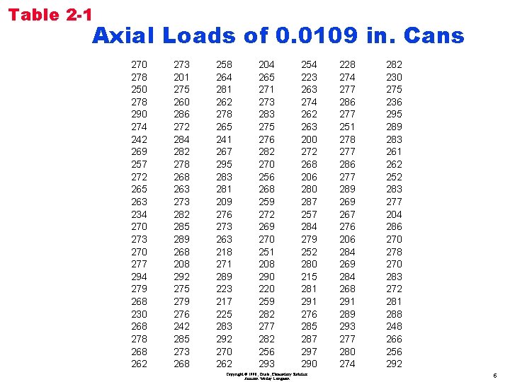
Table 2 -1 Axial Loads of 0. 0109 in. Cans 270 278 250 278 290 274 242 269 257 272 265 263 234 270 273 270 277 294 279 268 230 268 278 262 273 201 275 260 286 272 284 282 278 263 273 282 285 289 268 208 292 275 279 276 242 285 273 268 258 264 281 262 278 265 241 267 295 283 281 209 276 273 263 218 271 289 223 217 225 283 292 270 262 204 265 271 273 283 275 276 282 270 256 268 259 272 269 270 251 208 290 220 259 282 277 282 256 293 254 223 263 274 262 263 200 272 268 206 280 287 257 284 279 252 280 215 281 291 276 285 287 290 Copyright © 1998, Triola, Elementary Statistics Addison Wesley Longman 228 274 277 286 277 251 278 277 286 277 289 267 276 206 284 269 284 268 291 289 293 277 280 274 282 230 275 236 295 289 283 261 262 252 283 277 204 286 270 278 270 283 272 281 288 248 266 256 292 5

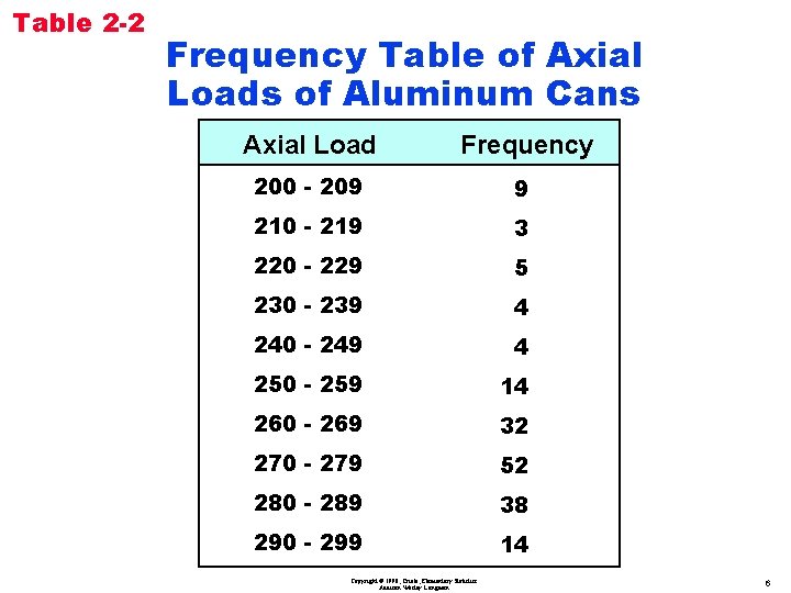
Table 2 -2 Frequency Table of Axial Loads of Aluminum Cans Axial Load Frequency 200 - 209 9 210 - 219 3 220 - 229 5 230 - 239 4 240 - 249 4 250 - 259 14 260 - 269 32 270 - 279 52 280 - 289 38 290 - 299 14 Copyright © 1998, Triola, Elementary Statistics Addison Wesley Longman 6

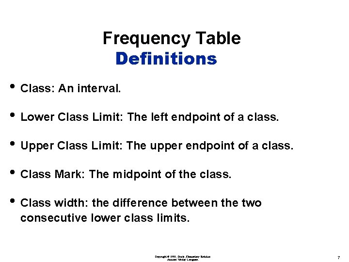
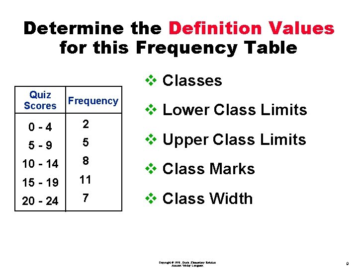
Frequency Table Definitions • Class: An interval. • Lower Class Limit: The left endpoint of a class. • Upper Class Limit: The upper endpoint of a class. • Class Mark: The midpoint of the class. • Class width: the difference between the two consecutive lower class limits. Copyright © 1998, Triola, Elementary Statistics Addison Wesley Longman 7

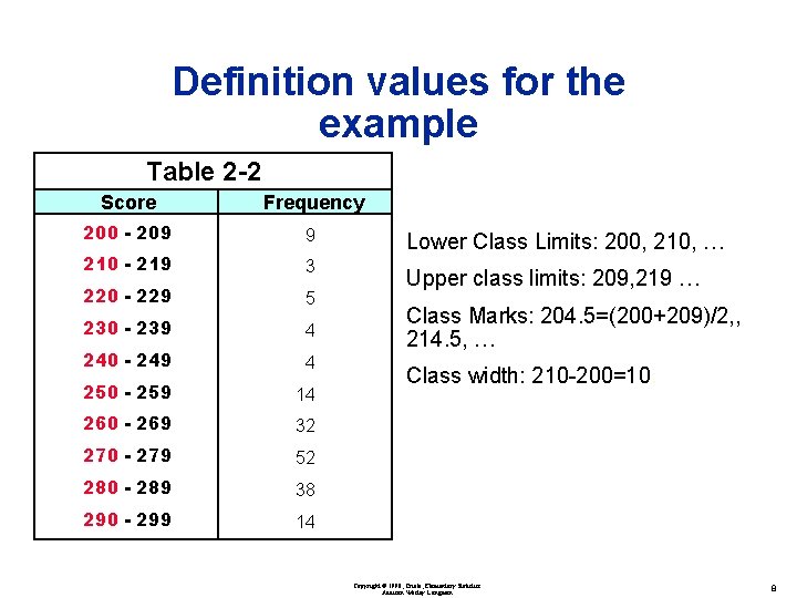
Definition values for the example Table 2 -2 Score Frequency 200 - 209 9 210 - 219 3 220 - 229 5 230 - 239 4 240 - 249 4 250 - 259 14 260 - 269 32 270 - 279 52 280 - 289 38 290 - 299 14 Lower Class Limits: 200, 210, … Upper class limits: 209, 219 … Class Marks: 204. 5=(200+209)/2, , 214. 5, … Class width: 210 -200=10. Copyright © 1998, Triola, Elementary Statistics Addison Wesley Longman 8

Determine the Definition Values for this Frequency Table v Classes Quiz Scores Frequency v Lower Class Limits 0 -4 2 5 -9 5 v Upper Class Limits 10 - 14 8 15 - 19 11 v Class Marks 20 - 24 7 v Class Width Copyright © 1998, Triola, Elementary Statistics Addison Wesley Longman 9

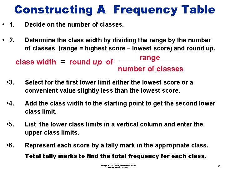
Constructing A Frequency Table • 1. Decide on the number of classes. • 2. Determine the class width by dividing the range by the number of classes (range = highest score – lowest score) and round up. class width = round up of range number of classes • 3. Select for the first lower limit either the lowest score or a convenient value slightly less than the lowest score. • 4. Add the class width to the starting point to get the second lower class limit. • 5. List the lower class limits in a vertical column and enter the upper class limits. • 6. Represent each score by a tally mark in the appropriate class. Total tally marks to find the total frequency for each class. Copyright © 1998, Triola, Elementary Statistics Addison Wesley Longman 10

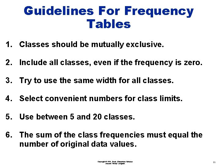
Guidelines For Frequency Tables 1. Classes should be mutually exclusive. 2. Include all classes, even if the frequency is zero. 3. Try to use the same width for all classes. 4. Select convenient numbers for class limits. 5. Use between 5 and 20 classes. 6. The sum of the class frequencies must equal the number of original data values. Copyright © 1998, Triola, Elementary Statistics Addison Wesley Longman 11

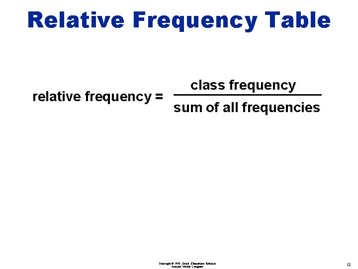
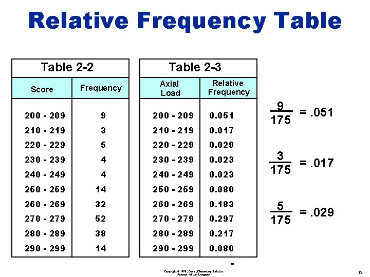
Relative Frequency Table relative frequency = class frequency sum of all frequencies Copyright © 1998, Triola, Elementary Statistics Addison Wesley Longman 12

Relative Frequency Table 2 -2 Score Table 2 -3 Frequency Axial Load Relative Frequency 200 - 209 9 200 - 209 0. 051 210 - 219 3 210 - 219 0. 017 220 - 229 5 220 - 229 0. 029 230 - 239 4 230 - 239 0. 023 240 - 249 4 240 - 249 0. 023 250 - 259 14 250 - 259 0. 080 260 - 269 32 260 - 269 0. 183 270 - 279 52 270 - 279 0. 297 280 - 289 38 280 - 289 0. 217 290 - 299 14 290 - 299 0. 080 9 =. 051 175 3 =. 017 175 5 =. 029 175 Copyright © 1998, Triola, Elementary Statistics Addison Wesley Longman 13

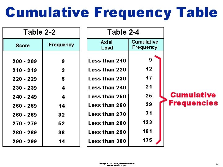
Cumulative Frequency Table 2 -2 Score Table 2 -4 Frequency Axial Load Cumulative Frequency 200 - 209 9 Less than 210 9 210 - 219 3 Less than 220 12 220 - 229 5 Less than 230 17 230 - 239 4 Less than 240 21 240 - 249 4 Less than 250 25 250 - 259 14 Less than 260 39 260 - 269 32 Less than 270 71 270 - 279 52 Less than 280 123 280 - 289 38 Less than 290 161 290 - 299 14 Less than 300 175 Copyright © 1998, Triola, Elementary Statistics Addison Wesley Longman Cumulative Frequencies 14

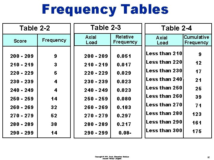
Frequency Tables Table 2 -3 Table 2 -2 Score Frequency Axial Load Relative Frequency 200 - 209 9 200 - 209 0. 051 210 - 219 3 210 - 219 0. 017 220 - 229 5 220 - 229 0. 029 230 - 239 4 230 - 239 0. 023 240 - 249 4 240 - 249 0. 023 250 - 259 14 250 - 259 0. 080 260 - 269 32 260 - 269 0. 183 270 - 279 52 270 - 279 0. 297 280 - 289 38 280 - 289 0. 217 290 - 299 14 290 - 299 0. 08 - Copyright © 1998, Triola, Elementary Statistics Addison Wesley Longman Table 2 -4 Axial Load Cumulative Frequency Less than 210 9 Less than 220 12 Less than 230 17 Less than 240 21 Less than 250 25 Less than 260 39 Less than 270 71 Less than 280 123 Less than 290 161 Less than 300 175 15

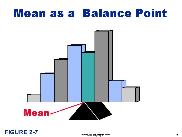
Mean as a Balance Point Mean FIGURE 2 -7 Copyright © 1998, Triola, Elementary Statistics Addison Wesley Longman 16

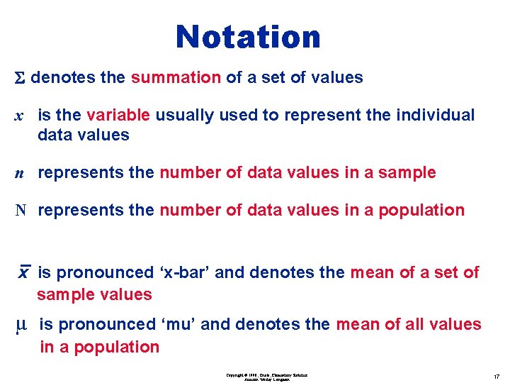
Notation S denotes the summation of a set of values x is the variable usually used to represent the individual data values n represents the number of data values in a sample N represents the number of data values in a population x is pronounced ‘x-bar’ and denotes the mean of a set of sample values µ is pronounced ‘mu’ and denotes the mean of all values in a population Copyright © 1998, Triola, Elementary Statistics Addison Wesley Longman 17

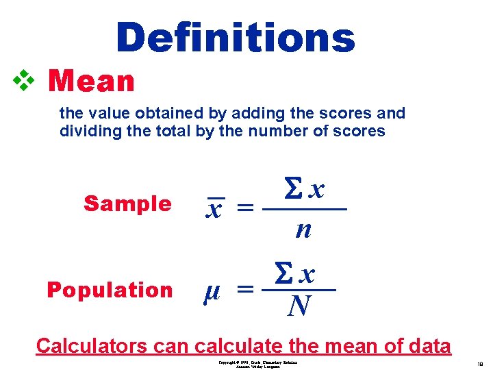
Definitions v Mean the value obtained by adding the scores and dividing the total by the number of scores Sample Population x = Sx n Sx µ = N Calculators can calculate the mean of data Copyright © 1998, Triola, Elementary Statistics Addison Wesley Longman 18

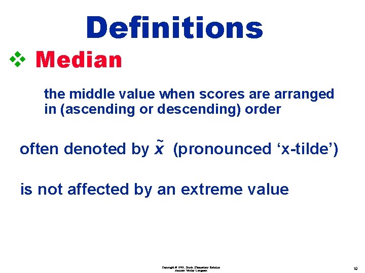
Definitions v Median the middle value when scores are arranged in (ascending or descending) order ~ often denoted by x (pronounced ‘x-tilde’) is not affected by an extreme value Copyright © 1998, Triola, Elementary Statistics Addison Wesley Longman 19

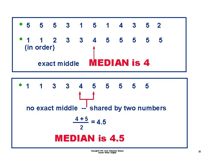
• • 5 5 5 3 1 5 1 4 3 5 2 1 1 2 (in order) 3 3 4 5 5 5 exact middle • 1 1 3 3 4 MEDIAN is 4 5 5 5 no exact middle -- shared by two numbers 4+5 2 = 4. 5 MEDIAN is 4. 5 Copyright © 1998, Triola, Elementary Statistics Addison Wesley Longman 20

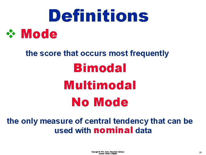
Definitions v Mode the score that occurs most frequently Bimodal Multimodal No Mode the only measure of central tendency that can be used with nominal data Copyright © 1998, Triola, Elementary Statistics Addison Wesley Longman 21

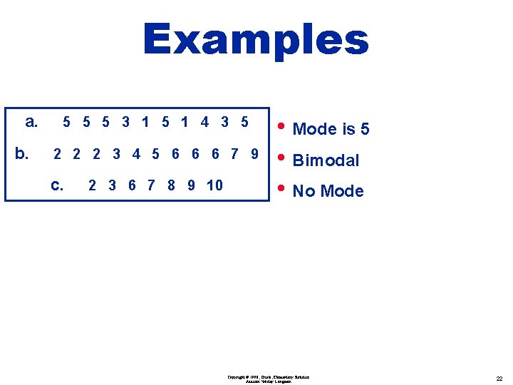
Examples a. b. 5 5 5 3 1 5 1 4 3 5 2 2 2 3 4 5 6 6 6 7 9 c. 2 3 6 7 8 9 10 • Mode is 5 • Bimodal • No Mode Copyright © 1998, Triola, Elementary Statistics Addison Wesley Longman 22

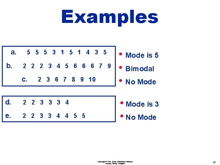
Examples a. b. 5 5 5 3 1 5 1 4 3 5 2 2 2 3 4 5 6 6 6 7 9 c. 2 3 6 7 8 9 10 d. 2 2 3 3 3 4 e. 2 2 3 3 4 4 5 5 • Mode is 5 • Bimodal • No Mode • Mode is 3 • No Mode Copyright © 1998, Triola, Elementary Statistics Addison Wesley Longman 23

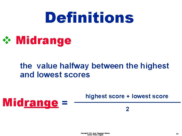
Definitions v Midrange the value halfway between the highest and lowest scores Midrange = highest score + lowest score 2 Copyright © 1998, Triola, Elementary Statistics Addison Wesley Longman 24

Round-off rule for measures of central tendency Carry one more decimal place than is present in the orignal set of data Copyright © 1998, Triola, Elementary Statistics Addison Wesley Longman 25

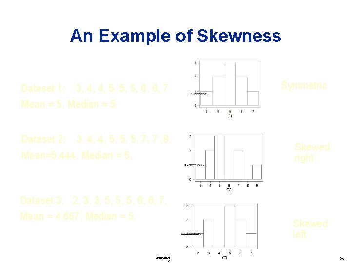
An Example of Skewness Dataset 1: 3, 4, 4, 5, 5, 5, 6, 6, 7 Symmetric Mean = 5, Median = 5 Dataset 2: 3, 4, 4, 5, 5, 5, 7, 7 , 9. Mean=5. 444, Median = 5. Skewed right Dataset 3: 2, 3, 3, 5, 5, 5, 6, 6, 7. Mean = 4. 667, Median = 5. Skewed left Copyright © 1998, Triola, Elementary Statistics Addison Wesley Longman 26

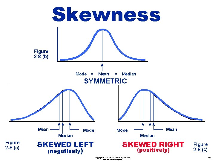
Skewness Figure 2 -8 (b) Mode = Mean = Median SYMMETRIC Mean Mode Median Figure 2 -8 (a) SKEWED LEFT (negatively) Mean Mode Median SKEWED RIGHT (positively) Copyright © 1998, Triola, Elementary Statistics Addison Wesley Longman Figure 2 -8 (c) 27

Best Measure of Central Tendency Table 2 -6 • Advantages - Disadvantages Copyright © 1998, Triola, Elementary Statistics Addison Wesley Longman 28

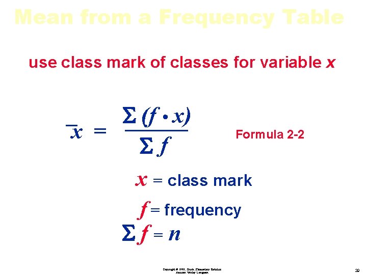
Mean from a Frequency Table use class mark of classes for variable x S (f • x) x = Formula 2 -2 Sf x = class mark f = frequency Sf=n Copyright © 1998, Triola, Elementary Statistics Addison Wesley Longman 29

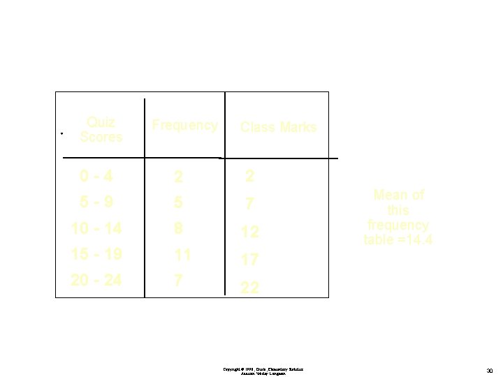
Quiz Scores Frequency Class Marks 0 -4 2 2 5 -9 5 7 10 - 14 8 12 15 - 19 11 17 20 - 24 7 22 Copyright © 1998, Triola, Elementary Statistics Addison Wesley Longman Mean of this frequency table =14. 4 30

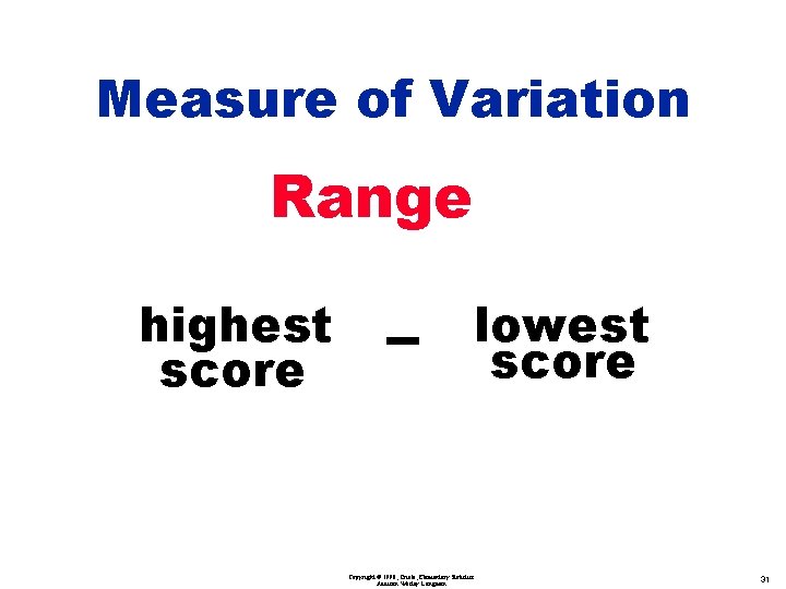
Measure of Variation Range highest score lowest score Copyright © 1998, Triola, Elementary Statistics Addison Wesley Longman 31

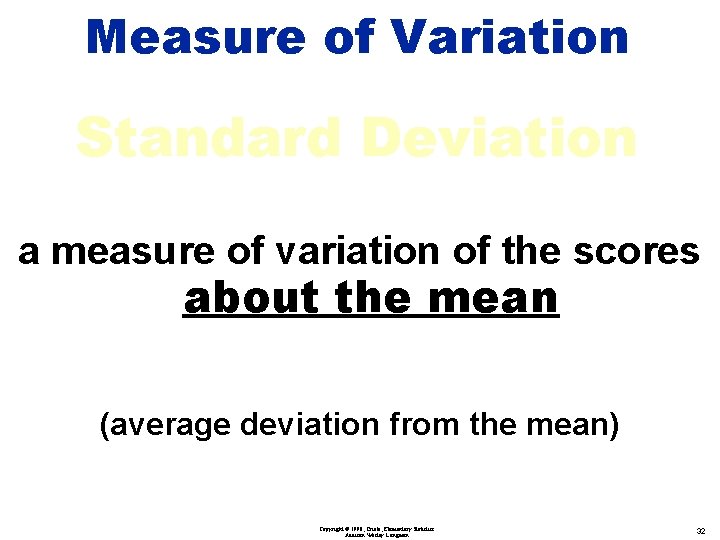
Measure of Variation Standard Deviation a measure of variation of the scores about the mean (average deviation from the mean) Copyright © 1998, Triola, Elementary Statistics Addison Wesley Longman 32

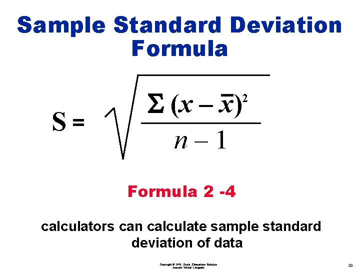
Sample Standard Deviation Formula S= S (x – x) n– 1 2 Formula 2 -4 calculators can calculate sample standard deviation of data Copyright © 1998, Triola, Elementary Statistics Addison Wesley Longman 33

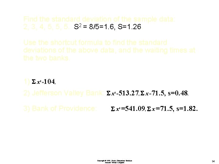
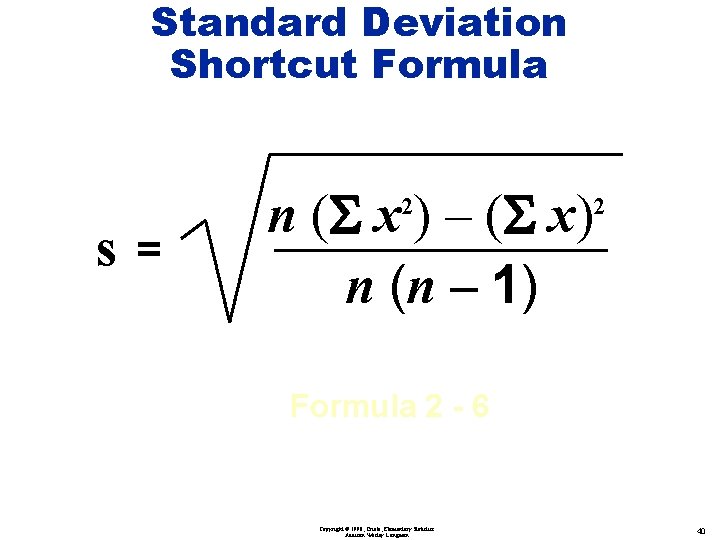
Find the standard deviation of the sample data: 2, 3, 4, 5, 5, 5. S 2 = 8/5=1. 6, S=1. 26. Use the shortcut formula to find the standard deviations of the above data, and the waiting times at the two banks. 1) S x =104, 2 2) Jefferson Valley Bank: S x =513. 27, S x =71. 5, s=0. 48. 2 3) Bank of Providence: Sx 2 =541. 09, S x =71. 5, s=1. 82. Copyright © 1998, Triola, Elementary Statistics Addison Wesley Longman 34

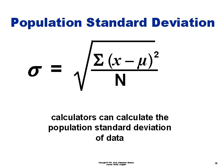
Population Standard Deviation s = S (x – µ) N 2 calculators can calculate the population standard deviation of data Copyright © 1998, Triola, Elementary Statistics Addison Wesley Longman 35

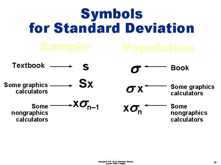
Symbols for Standard Deviation Sample Textbook Some graphics calculators Some nongraphics calculators Population s s Sx xsn– 1 sx x sn Copyright © 1998, Triola, Elementary Statistics Addison Wesley Longman Book Some graphics calculators Some nongraphics calculators 36

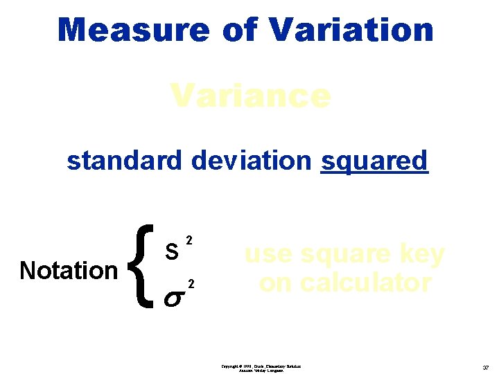
Measure of Variation Variance standard deviation squared } Notation s 2 use square key on calculator Copyright © 1998, Triola, Elementary Statistics Addison Wesley Longman 37

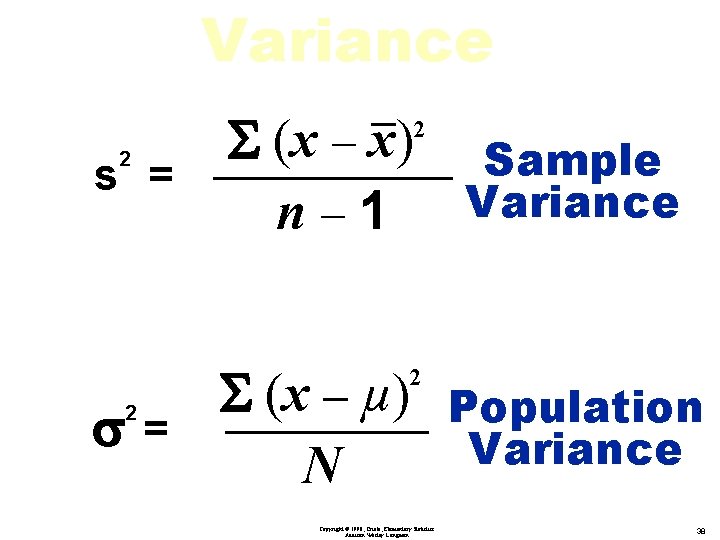
Variance S (x – x) Sample n – 1 Variance 2 2 s = S (x – µ) Population s= Variance N 2 2 Copyright © 1998, Triola, Elementary Statistics Addison Wesley Longman 38

Round-off Rule for measures of variation Carry one more decimal place than was present in the original data Copyright © 1998, Triola, Elementary Statistics Addison Wesley Longman 39

Standard Deviation Shortcut Formula s= n (S x ) – (S x) n (n – 1) 2 2 Formula 2 - 6 Copyright © 1998, Triola, Elementary Statistics Addison Wesley Longman 40

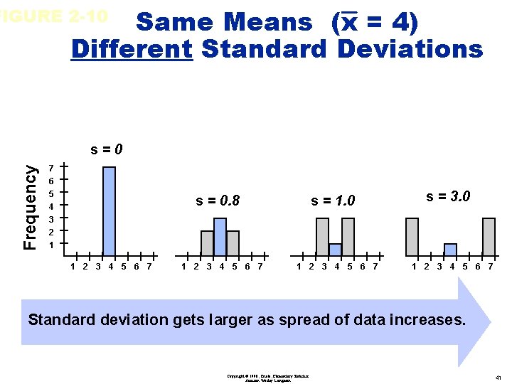
Same Means (x = 4) Different Standard Deviations FIGURE 2 -10 Frequency s=0 7 6 5 4 3 2 1 s = 0. 8 1 2 3 4 5 6 7 s = 1. 0 1 2 3 4 5 6 7 s = 3. 0 1 2 3 4 5 6 7 Standard deviation gets larger as spread of data increases. Copyright © 1998, Triola, Elementary Statistics Addison Wesley Longman 41

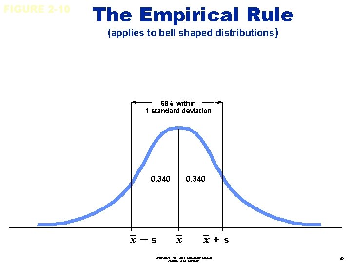
FIGURE 2 -10 The Empirical Rule (applies to bell shaped distributions) 68% within 1 standard deviation 0. 340 x–s 0. 340 x x+s Copyright © 1998, Triola, Elementary Statistics Addison Wesley Longman 42

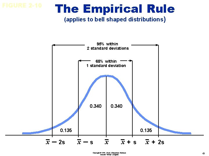
FIGURE 2 -10 The Empirical Rule (applies to bell shaped distributions) 95% within 2 standard deviations 68% within 1 standard deviation 0. 340 0. 135 x – 2 s 0. 135 x–s x x+s Copyright © 1998, Triola, Elementary Statistics Addison Wesley Longman x + 2 s 43

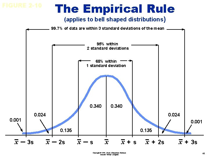
FIGURE 2 -10 The Empirical Rule (applies to bell shaped distributions) 99. 7% of data are within 3 standard deviations of the mean 95% within 2 standard deviations 68% within 1 standard deviation 0. 340 0. 024 0. 001 0. 135 x – 3 s x – 2 s 0. 135 x–s x x+s Copyright © 1998, Triola, Elementary Statistics Addison Wesley Longman x + 2 s x + 3 s 44

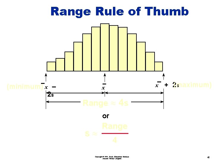
Range Rule of Thumb (minimum) x – 2 s x x + 2(maximum) s Range » 4 s or s» Range 4 Copyright © 1998, Triola, Elementary Statistics Addison Wesley Longman 45

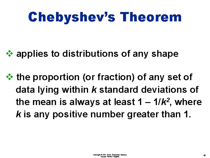
Chebyshev’s Theorem v applies to distributions of any shape v the proportion (or fraction) of any set of data lying within k standard deviations of the mean is always at least 1 – 1/k 2, where k is any positive number greater than 1. Copyright © 1998, Triola, Elementary Statistics Addison Wesley Longman 46

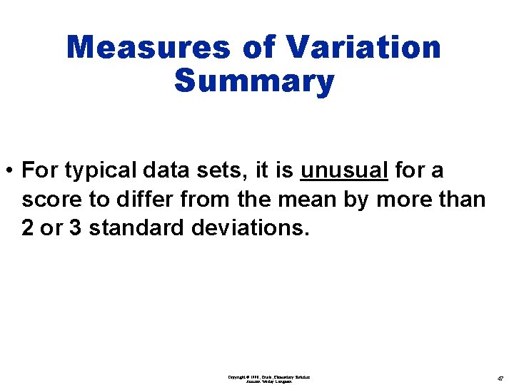
Measures of Variation Summary • For typical data sets, it is unusual for a score to differ from the mean by more than 2 or 3 standard deviations. Copyright © 1998, Triola, Elementary Statistics Addison Wesley Longman 47

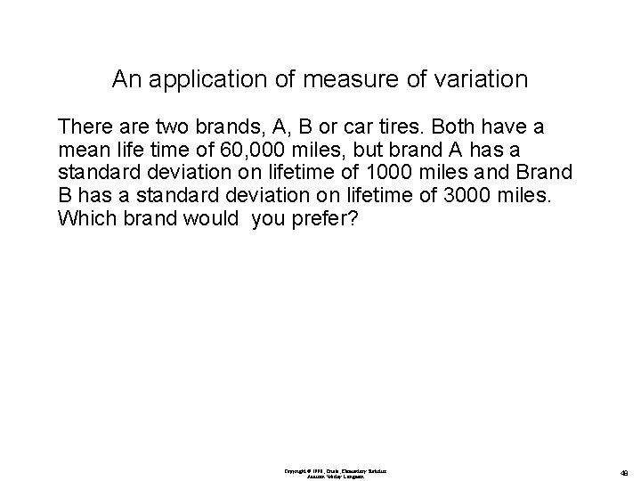
An application of measure of variation There are two brands, A, B or car tires. Both have a mean life time of 60, 000 miles, but brand A has a standard deviation on lifetime of 1000 miles and Brand B has a standard deviation on lifetime of 3000 miles. Which brand would you prefer? Copyright © 1998, Triola, Elementary Statistics Addison Wesley Longman 48

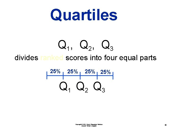
Quartiles Q 1, Q 2, Q 3 divides ranked scores into four equal parts 25% 25% Q 1 Q 2 Q 3 Copyright © 1998, Triola, Elementary Statistics Addison Wesley Longman 49

Percentiles • 99 Percentiles Copyright © 1998, Triola, Elementary Statistics Addison Wesley Longman 50

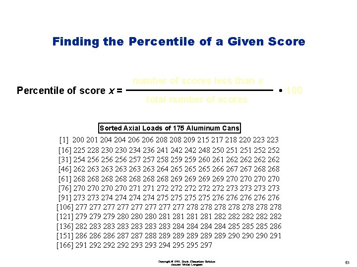
Finding the Percentile of a Given Score Percentile of score x = number of scores less than x total number of scores • 100 Sorted Axial Loads of 175 Aluminum Cans [1] 200 201 204 206 208 209 215 217 218 220 223 [16] 225 228 230 234 236 241 242 248 250 251 252 [31] 254 256 256 257 258 259 260 261 262 262 [46] 262 263 263 263 264 265 265 266 267 268 [61] 268 268 269 269 270 270 [76] 270 270 271 272 272 272 273 273 [91] 273 274 274 275 275 276 276 276 [106] 277 277 278 278 [121] 279 279 280 280 281 281 282 282 282 [136] 282 283 283 283 284 284 285 285 286 [151] 286 286 287 288 289 289 289 290 290 291 [166] 291 292 292 293 294 295 297 Copyright © 1998, Triola, Elementary Statistics Addison Wesley Longman 51

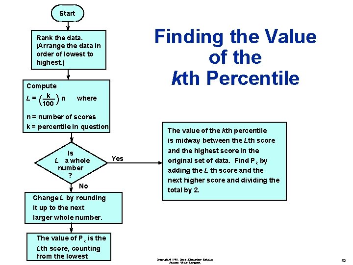
Start Finding the Value of the kth Percentile Rank the data. (Arrange the data in order of lowest to highest. ) Compute L= k n 100 ( ) where n = number of scores k = percentile in question Is L a whole number ? No Change L by rounding it up to the next larger whole number. The value of Pk is the Lth score, counting from the lowest Yes The value of the kth percentile is midway between the Lth score and the highest score in the original set of data. Find Pk by adding the L th score and the next higher score and dividing the total by 2. Copyright © 1998, Triola, Elementary Statistics Addison Wesley Longman 52
![Sorted Axial Loads of 175 Aluminum Cans 1 200 201 204 206 208 209 Sorted Axial Loads of 175 Aluminum Cans [1] 200 201 204 206 208 209](https://slidetodoc.com/presentation_image_h2/1f3a22e771f810e8a22069c2a0991fa2/image-53.jpg)
Sorted Axial Loads of 175 Aluminum Cans [1] 200 201 204 206 208 209 215 217 218 220 223 [16] 225 228 230 234 236 241 242 248 250 251 252 [31] 254 256 256 257 258 259 260 261 262 262 [46] 262 263 263 263 264 265 265 266 267 268 [61] 268 268 269 269 270 270 [76] 270 270 271 272 272 272 273 273 [91] 273 274 274 275 275 276 276 276 [106] 277 277 278 278 [121] 279 279 280 280 281 281 282 282 282 [136] 282 283 283 283 284 284 285 285 286 [151] 286 286 287 288 289 289 289 290 290 291 [166] 291 292 292 293 294 295 297 The 10 th percentile: L=175*10/100=17. 5, round up to 18. So the 10 th percentile is the 18 th one in the sorted data, i. e. , 230. The 25 th percentile: L=175*25/100=43. 52, rounded up to 44. The 25 th percentile is the 44 th one in the sorted data, I. ei. 262. Copyright © 1998, Triola, Elementary Statistics Addison Wesley Longman 53

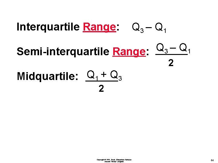
Interquartile Range: Q 3 – Q 1 Semi-interquartile Range: Q 3 – Q 1 2 Midquartile: Q 1 + Q 3 2 Copyright © 1998, Triola, Elementary Statistics Addison Wesley Longman 54

Exploratory Data Analysis v Used to explore data at a preliminary level v Few or no assumptions are made about the data v Tends to evolve relatively simple calculations and graphs Copyright © 1998, Triola, Elementary Statistics Addison Wesley Longman 55

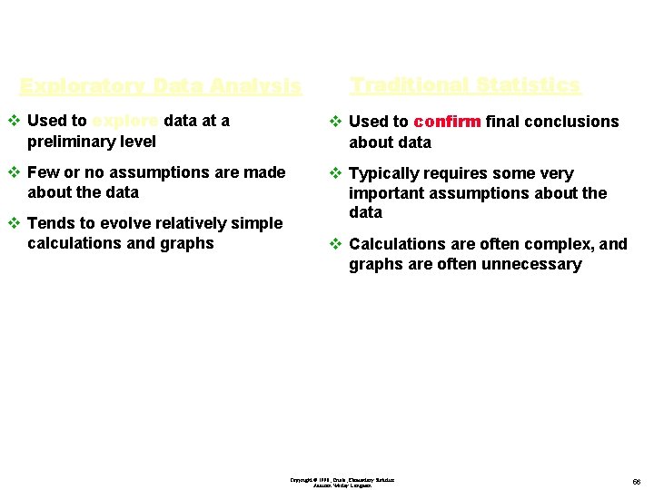
Exploratory Data Analysis Traditional Statistics v Used to explore data at a preliminary level v Used to confirm final conclusions about data v Few or no assumptions are made about the data v Typically requires some very important assumptions about the data v Tends to evolve relatively simple calculations and graphs v Calculations are often complex, and graphs are often unnecessary Copyright © 1998, Triola, Elementary Statistics Addison Wesley Longman 56

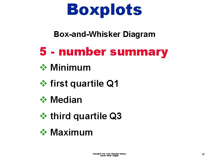
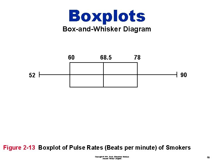
Boxplots Box-and-Whisker Diagram 5 - number summary v Minimum v first quartile Q 1 v Median v third quartile Q 3 v Maximum Copyright © 1998, Triola, Elementary Statistics Addison Wesley Longman 57

Boxplots Box-and-Whisker Diagram 60 68. 5 78 90 52 Figure 2 -13 Boxplot of Pulse Rates (Beats per minute) of Smokers Copyright © 1998, Triola, Elementary Statistics Addison Wesley Longman 58

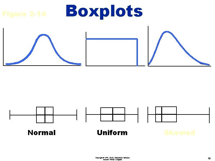
Figure 2 -14 Normal Boxplots Uniform Copyright © 1998, Triola, Elementary Statistics Addison Wesley Longman Skewed 59

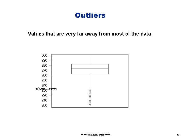
Outliers Values that are very far away from most of the data Copyright © 1998, Triola, Elementary Statistics Addison Wesley Longman 60

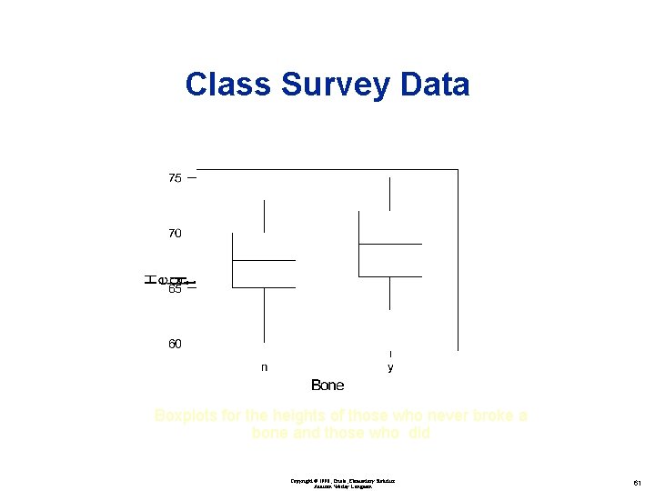
Class Survey Data Boxplots for the heights of those who never broke a bone and those who did Copyright © 1998, Triola, Elementary Statistics Addison Wesley Longman 61

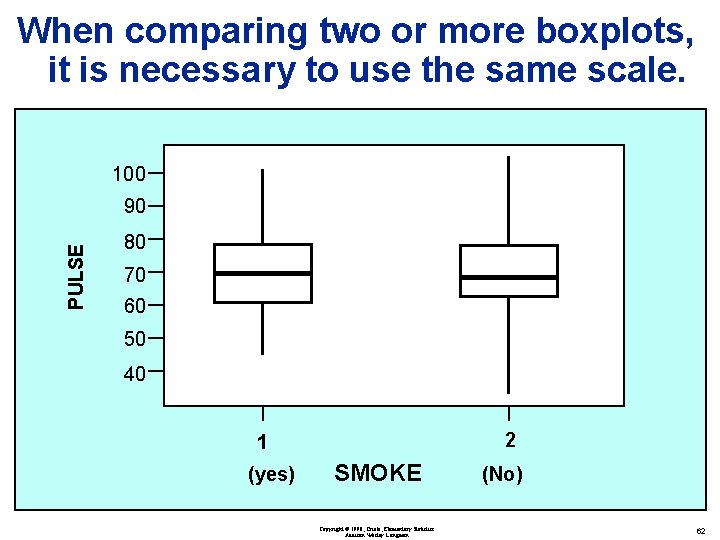
When comparing two or more boxplots, it is necessary to use the same scale. 100 PULSE 90 80 70 60 50 40 2 1 (yes) SMOKE Copyright © 1998, Triola, Elementary Statistics Addison Wesley Longman (No) 62