Chapter 2 Descriptive Statistics 1 LarsonFarber 4 th

Chapter 2 Descriptive Statistics 1 Larson/Farber 4 th ed.

Useful screencast/videos: �Video on creating a frequency distribution by hand: http: //screencast. com/t/OGY 3 Zj. Jj �Video on using Excel 2007 to create frequency distributions: http: //screencast. com/t/tk. Mv 2 FMWh. Je �Video on using Excel 2007 to create a histogram http: //screencast. com/t/L 0 u 9 UI 2 e. I Larson/Farber 4 th ed. 2

Section 2. 1 Frequency Distributions and Their Graphs 3 Larson/Farber 4 th ed.

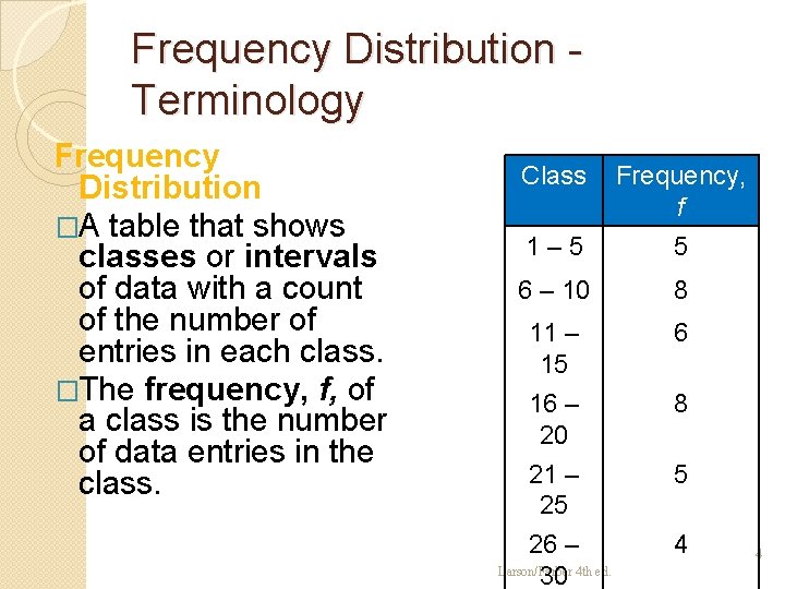
Frequency Distribution Terminology Frequency Distribution �A table that shows classes or intervals of data with a count of the number of entries in each class. �The frequency, f, of a class is the number of data entries in the class. Class Frequency, f 1– 5 5 6 – 10 8 11 – 15 16 – 20 6 21 – 25 26 – Larson/Farber 4 th ed. 30 5 8 4 4

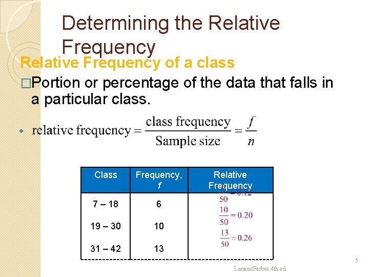
Determining the Relative Frequency of a class �Portion or percentage of the data that falls in a particular class. • Class Frequency, f 7 – 18 6 19 – 30 10 31 – 42 13 Relative Frequency 5 Larson/Farber 4 th ed.

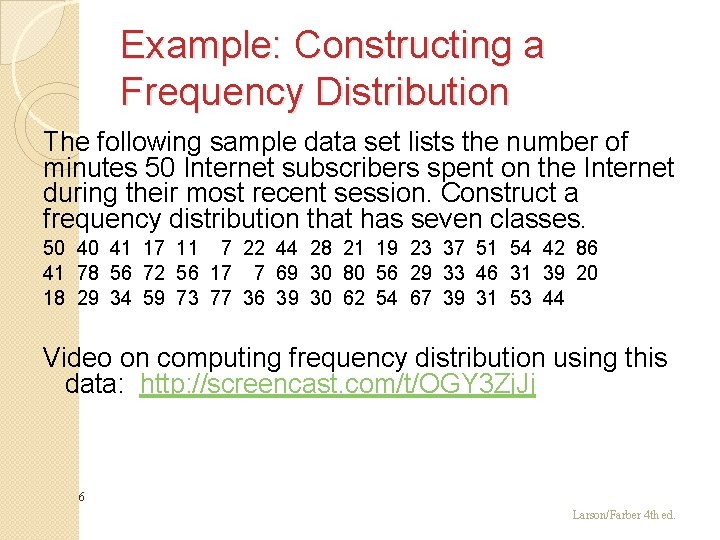
Example: Constructing a Frequency Distribution The following sample data set lists the number of minutes 50 Internet subscribers spent on the Internet during their most recent session. Construct a frequency distribution that has seven classes. 50 40 41 17 11 7 22 44 28 21 19 23 37 51 54 42 86 41 78 56 72 56 17 7 69 30 80 56 29 33 46 31 39 20 18 29 34 59 73 77 36 39 30 62 54 67 39 31 53 44 Video on computing frequency distribution using this data: http: //screencast. com/t/OGY 3 Zj. Jj 6 Larson/Farber 4 th ed.

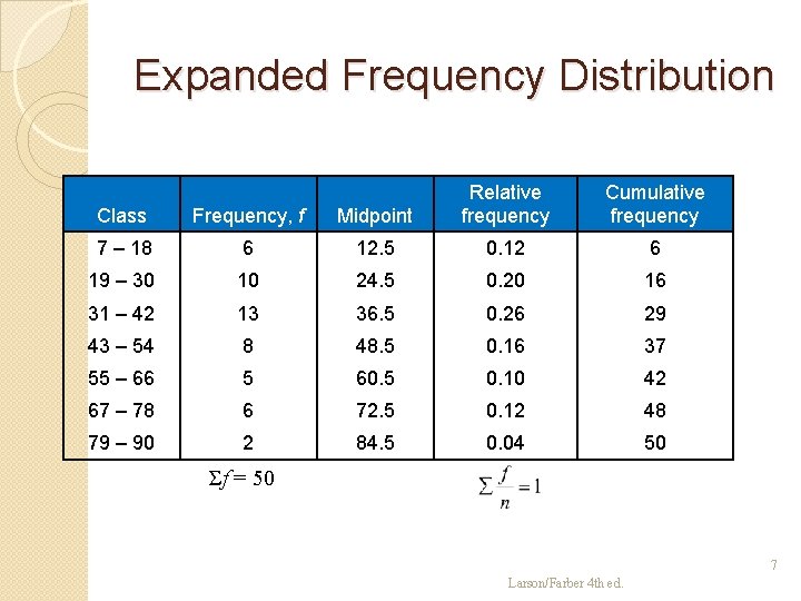
Expanded Frequency Distribution Class Frequency, f Midpoint Relative frequency Cumulative frequency 7 – 18 6 12. 5 0. 12 6 19 – 30 10 24. 5 0. 20 16 31 – 42 13 36. 5 0. 26 29 43 – 54 8 48. 5 0. 16 37 55 – 66 5 60. 5 0. 10 42 67 – 78 6 72. 5 0. 12 48 79 – 90 2 84. 5 0. 04 50 Σf = 50 7 Larson/Farber 4 th ed.

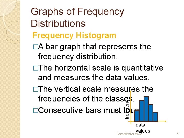
Graphs of Frequency Distributions frequency Frequency Histogram �A bar graph that represents the frequency distribution. �The horizontal scale is quantitative and measures the data values. �The vertical scale measures the frequencies of the classes. �Consecutive bars must touch. data values Larson/Farber 4 th ed. 8

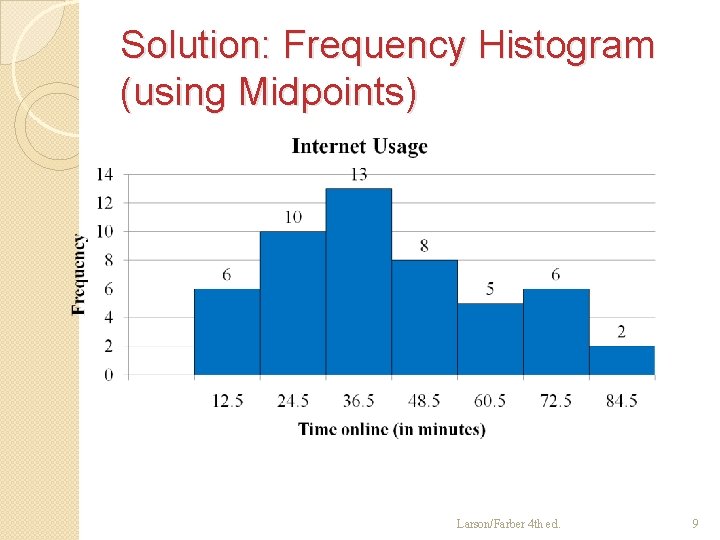
Solution: Frequency Histogram (using Midpoints) Larson/Farber 4 th ed. 9

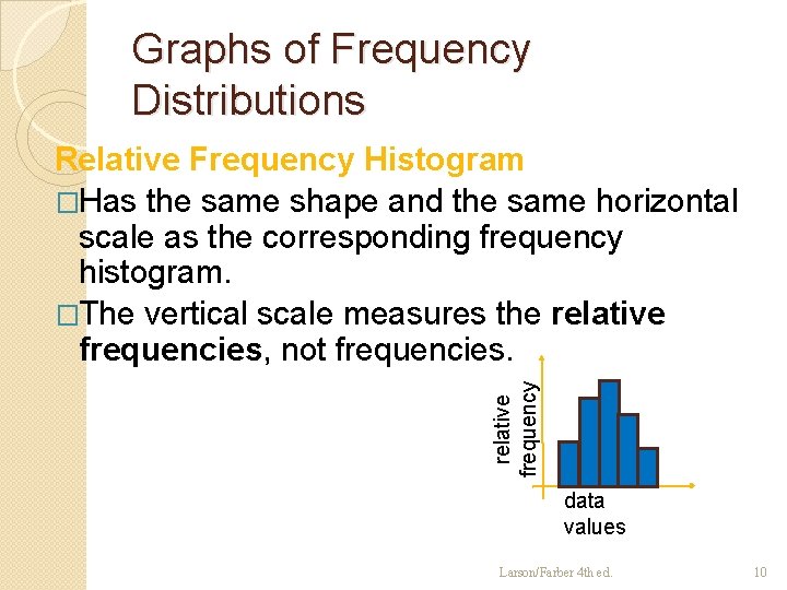
Graphs of Frequency Distributions relative frequency Relative Frequency Histogram �Has the same shape and the same horizontal scale as the corresponding frequency histogram. �The vertical scale measures the relative frequencies, not frequencies. data values Larson/Farber 4 th ed. 10

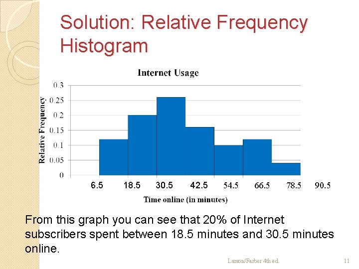
Solution: Relative Frequency Histogram 6. 5 18. 5 30. 5 42. 5 54. 5 66. 5 78. 5 90. 5 From this graph you can see that 20% of Internet subscribers spent between 18. 5 minutes and 30. 5 minutes online. Larson/Farber 4 th ed. 11

Section 2. 2 More Graphs and Displays Larson/Farber 4 th ed. 12

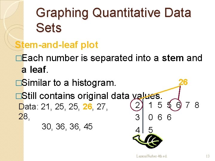
Graphing Quantitative Data Sets Stem-and-leaf plot �Each number is separated into a stem and a leaf. 26 �Similar to a histogram. �Still contains original data values. Data: 21, 25, 26, 27, 28, 30, 36, 45 2 3 1 5 5 6 7 8 0 6 6 4 5 Larson/Farber 4 th ed. 13

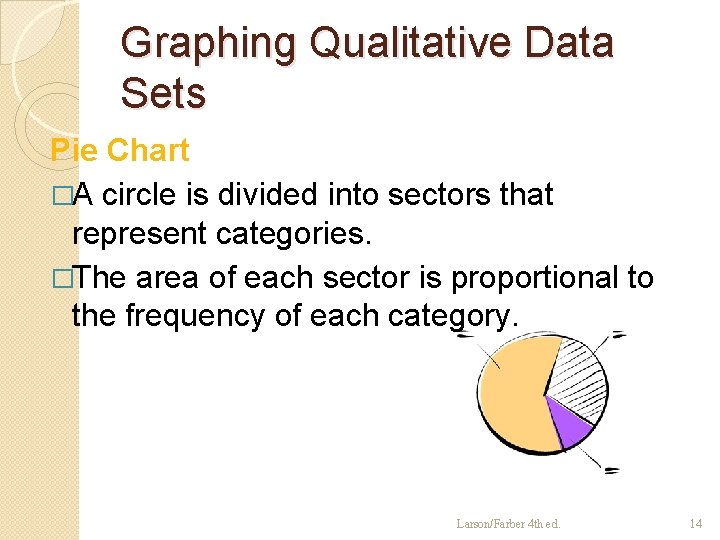
Graphing Qualitative Data Sets Pie Chart �A circle is divided into sectors that represent categories. �The area of each sector is proportional to the frequency of each category. Larson/Farber 4 th ed. 14

Section 2. 3 Measures of Central Tendency Larson/Farber 4 th ed. 15

Measures of Central Tendency Measure of central tendency �A value that represents a typical, or central, entry of a data set. �Most common measures of central tendency: ◦ Mean ◦ Median ◦ Mode Larson/Farber 4 th ed. 16

Measure of Central Tendency: Mean (average) �The sum of all the data entries divided by the number of entries. �Sigma notation: Σx = add all of the data entries (x) in the data set. �Population mean: �Sample mean: Larson/Farber 4 th ed. 17

Example: Finding a Sample Mean The prices (in dollars) for a sample of roundtrip flights from Chicago, Illinois to Cancun, Mexico are listed. What is the mean price of the flights? 872 432 397 427 388 782 397 Larson/Farber 4 th ed. 18

Solution: Finding a Sample Mean 872 432 397 427 388 782 397 • The sum of the flight prices is Σx = 872 + 432 + 397 + 427 + 388 + 782 + 397 = 3695 • To find the mean price, divide the sum of the prices by the number of prices in the sample The mean price of the flights is about $527. 90. Larson/Farber 4 th ed. 19

Measure of Central Tendency: Median �The value that lies in the middle of the data when the data set is ordered. �Measures the center of an ordered data set by dividing it into two equal parts. �If the data set has an ◦ odd number of entries: median is the middle data entry. ◦ even number of entries: median is the mean of the two middle data entries. Larson/Farber 4 th ed. 20

Example: Finding the Median The prices (in dollars) for a sample of roundtrip flights from Chicago, Illinois to Cancun, Mexico are listed. Find the median of the flight prices. 872 432 397 427 388 782 397 Larson/Farber 4 th ed. 21

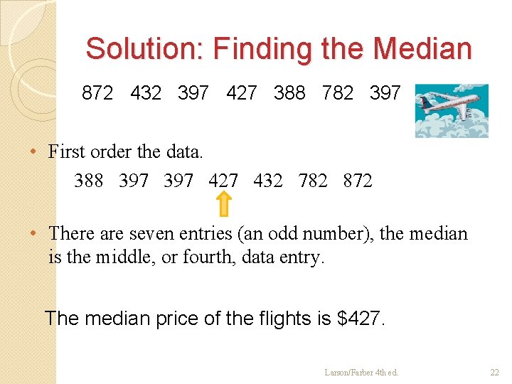
Solution: Finding the Median 872 432 397 427 388 782 397 • First order the data. 388 397 427 432 782 872 • There are seven entries (an odd number), the median is the middle, or fourth, data entry. The median price of the flights is $427. Larson/Farber 4 th ed. 22

Example: Finding the Median The flight priced at $432 is no longer available. What is the median price of the remaining flights? 872 397 427 388 782 397 Larson/Farber 4 th ed. 23

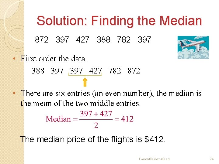
Solution: Finding the Median 872 397 427 388 782 397 • First order the data. 388 397 427 782 872 • There are six entries (an even number), the median is the mean of the two middle entries. The median price of the flights is $412. Larson/Farber 4 th ed. 24

Measure of Central Tendency: Mode �The data entry that occurs with the greatest frequency. �If no entry is repeated the data set has no mode. �If two entries occur with the same greatest frequency, each entry is a mode (bimodal). Larson/Farber 4 th ed. 25

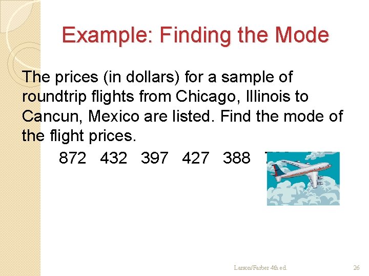
Example: Finding the Mode The prices (in dollars) for a sample of roundtrip flights from Chicago, Illinois to Cancun, Mexico are listed. Find the mode of the flight prices. 872 432 397 427 388 782 397 Larson/Farber 4 th ed. 26

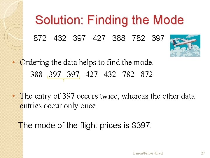
Solution: Finding the Mode 872 432 397 427 388 782 397 • Ordering the data helps to find the mode. 388 397 427 432 782 872 • The entry of 397 occurs twice, whereas the other data entries occur only once. The mode of the flight prices is $397. Larson/Farber 4 th ed. 27

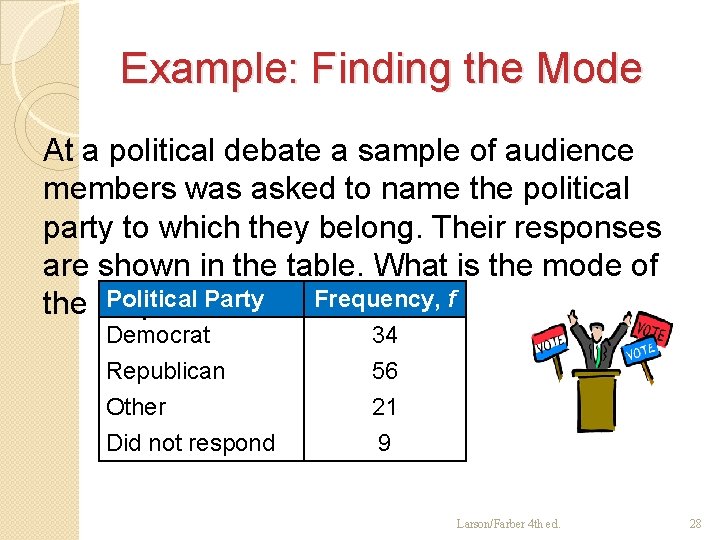
Example: Finding the Mode At a political debate a sample of audience members was asked to name the political party to which they belong. Their responses are shown in the table. What is the mode of Political Party Frequency, f the responses? Democrat Republican Other 34 56 21 Did not respond 9 Larson/Farber 4 th ed. 28

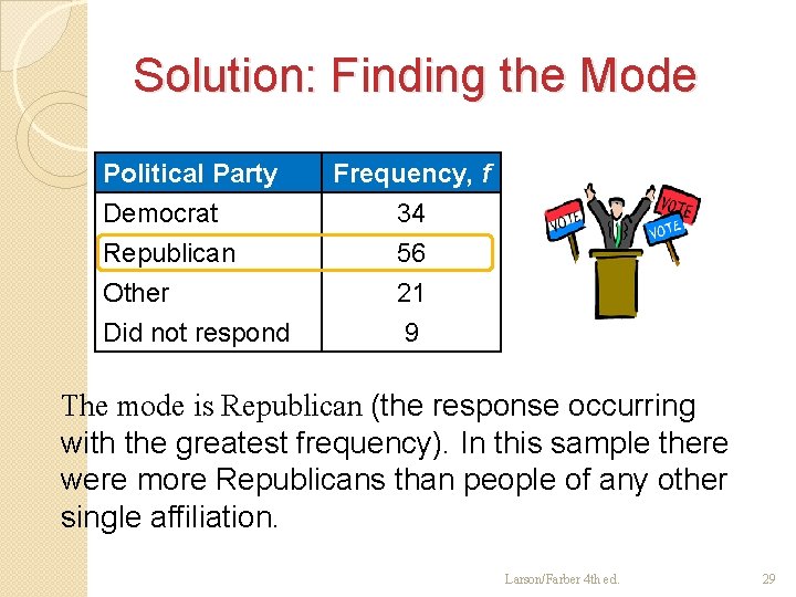
Solution: Finding the Mode Political Party Democrat Republican Other Frequency, f 34 56 21 Did not respond 9 The mode is Republican (the response occurring with the greatest frequency). In this sample there were more Republicans than people of any other single affiliation. Larson/Farber 4 th ed. 29

Section 2. 4 Measures of Variation Larson/Farber 4 th ed. 30

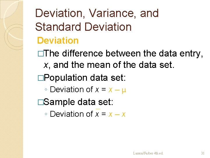
Deviation, Variance, and Standard Deviation �The difference between the data entry, x, and the mean of the data set. �Population data set: ◦ Deviation of x = x – μ �Sample data set: ◦ Deviation of x = x – x Larson/Farber 4 th ed. 31

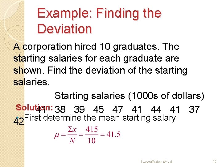
Example: Finding the Deviation A corporation hired 10 graduates. The starting salaries for each graduate are shown. Find the deviation of the starting salaries. Starting salaries (1000 s of dollars) Solution: 41 38 39 45 47 41 44 41 37 • First determine the mean starting salary. 42 Larson/Farber 4 th ed. 32

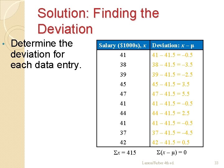
Solution: Finding the Deviation • Determine the deviation for each data entry. Salary ($1000 s), x Deviation: x – μ 41 41 – 41. 5 = – 0. 5 38 38 – 41. 5 = – 3. 5 39 39 – 41. 5 = – 2. 5 45 45 – 41. 5 = 3. 5 47 47 – 41. 5 = 5. 5 41 41 – 41. 5 = – 0. 5 44 44 – 41. 5 = 2. 5 41 41 – 41. 5 = – 0. 5 37 37 – 41. 5 = – 4. 5 42 42 – 41. 5 = 0. 5 Σx = 415 Σ(x – μ) = 0 Larson/Farber 4 th ed. 33

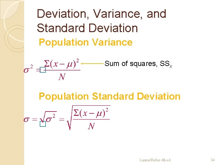
Deviation, Variance, and Standard Deviation Population Variance � Sum of squares, SSx Population Standard Deviation � Larson/Farber 4 th ed. 34

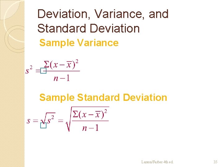
Deviation, Variance, and Standard Deviation Sample Variance � Sample Standard Deviation � Larson/Farber 4 th ed. 35

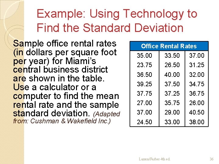
Example: Using Technology to Find the Standard Deviation Sample office rental rates (in dollars per square foot per year) for Miami’s central business district are shown in the table. Use a calculator or a computer to find the mean rental rate and the sample standard deviation. (Adapted from: Cushman & Wakefield Inc. ) Office Rental Rates 35. 00 33. 50 37. 00 23. 75 26. 50 31. 25 36. 50 40. 00 32. 00 39. 25 37. 50 34. 75 37. 25 36. 75 27. 00 35. 75 26. 00 37. 00 29. 00 40. 50 24. 50 33. 00 38. 00 Larson/Farber 4 th ed. 36

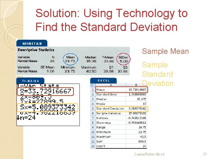
Solution: Using Technology to Find the Standard Deviation Sample Mean Sample Standard Deviation Larson/Farber 4 th ed. 37

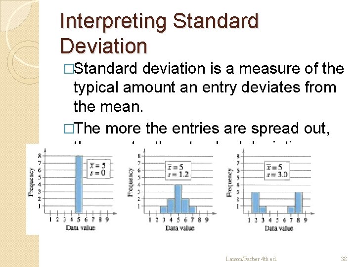
Interpreting Standard Deviation �Standard deviation is a measure of the typical amount an entry deviates from the mean. �The more the entries are spread out, the greater the standard deviation. Larson/Farber 4 th ed. 38

Interpreting Standard Deviation: Empirical Rule (68 – 95 – 99. 7 Rule) For data with a (symmetric) bell-shaped distribution, the standard deviation has the following characteristics: • About 68% of the data lie within one standard deviation of the mean. • About 95% of the data lie within two standard deviations of the mean. • About 99. 7% of the data lie within three standard deviations of the mean. Larson/Farber 4 th ed. 39

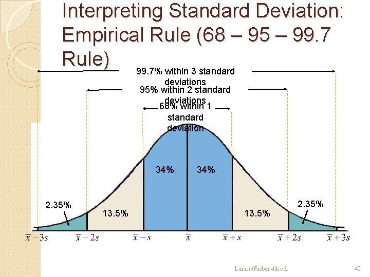
Interpreting Standard Deviation: Empirical Rule (68 – 95 – 99. 7 Rule) 99. 7% within 3 standard deviations 95% within 2 standard deviations 68% within 1 standard deviation 34% 2. 35% 13. 5% 34% 13. 5% Larson/Farber 4 th ed. 2. 35% 40

Example: Using the Empirical Rule In a survey conducted by the National Center for Health Statistics, the sample mean height of women in the United States (ages 20 -29) was 64 inches, with a sample standard deviation of 2. 71 inches. Estimate the percent of the women whose heights are between 64 inches and 69. 42 inches. Larson/Farber 4 th ed. 41

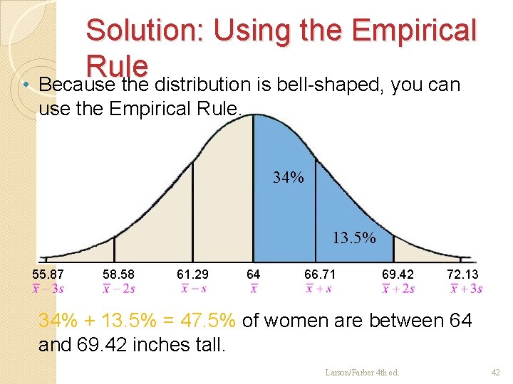
Solution: Using the Empirical Rule • Because the distribution is bell-shaped, you can use the Empirical Rule. 34% 13. 5% 55. 87 58. 58 61. 29 64 66. 71 69. 42 72. 13 34% + 13. 5% = 47. 5% of women are between 64 and 69. 42 inches tall. Larson/Farber 4 th ed. 42

Larson/Farber 4 th ed. 43

Larson/Farber 4 th ed. 44

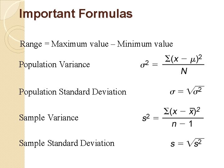
Important Formulas Range = Maximum value – Minimum value Population Variance Population Standard Deviation Sample Variance Sample Standard Deviation

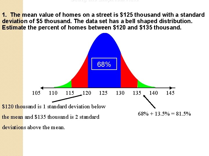
Using the Empirical Rule 1. The mean value of homes on a street is $125 thousand with a standard deviation of $5 thousand. The data set has a bell shaped distribution. Estimate the percent of homes between $120 and $135 thousand. 105 110 115 120 125 130 135 140 145 $120 thousand is 1 standard deviation below the mean and $135 thousand is 2 standard deviations above the mean. 68% + 13. 5% = 81. 5%

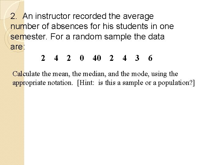
2. An instructor recorded the average number of absences for his students in one semester. For a random sample the data are: 2 4 2 0 40 2 4 3 6 Calculate the mean, the median, and the mode, using the appropriate notation. [Hint: is this a sample or a population? ]

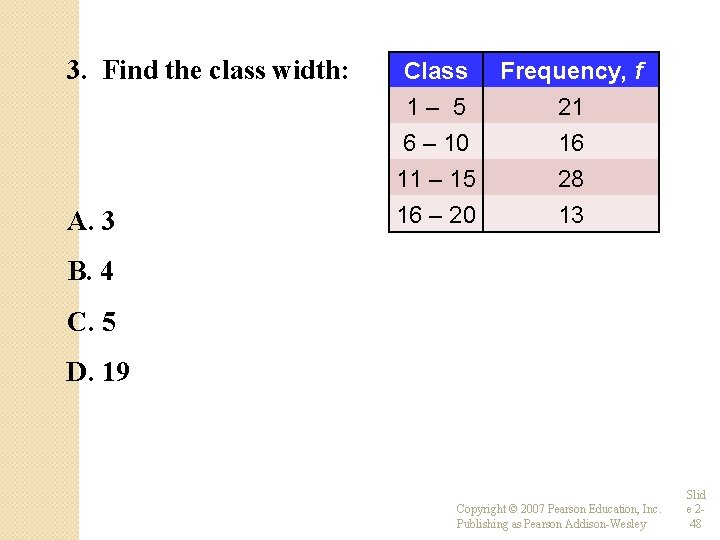
3. Find the class width: A. 3 Class Frequency, f 1– 5 6 –

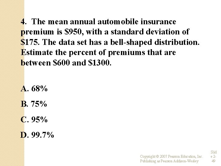
4. The mean annual automobile insurance premium is $950, with a standard deviation of $175. The data set has a bell-shaped distribution. Estimate the percent of premiums that are between $600 and $1300. A. 68% B. 75% C. 95% D. 99. 7% Copyright © 2007 Pearson Education, Inc. Publishing as Pearson Addison-Wesley Slid e 249

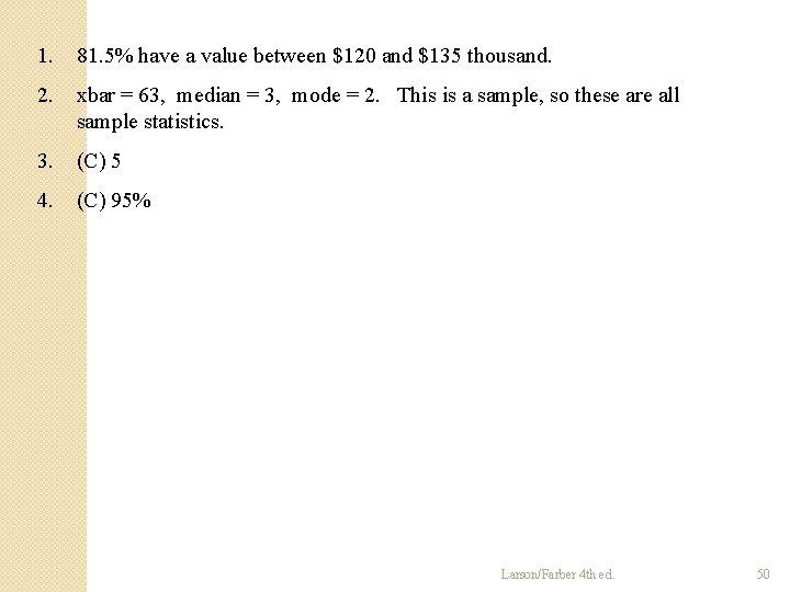
1. 81. 5% have a value between $120 and $135 thousand. 2. xbar = 63, median = 3, mode = 2. This is a sample, so these are all sample statistics. 3. (C) 5 4. (C) 95% Larson/Farber 4 th ed. 50