Chapter 2 Describing Data with Numerical Measures Graphical

Chapter 2: Describing Data with Numerical Measures Graphical methods may not always be sufficient for describing data. n Numerical measures can be created for both populations and samples. n A parameter is a numerical descriptive measure calculated for a population. • A statistic is a numerical descriptive measure calculated for a sample. •

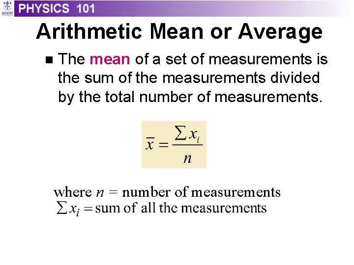
Arithmetic Mean or Average n The mean of a set of measurements is the sum of the measurements divided by the total number of measurements. where n = number of measurements

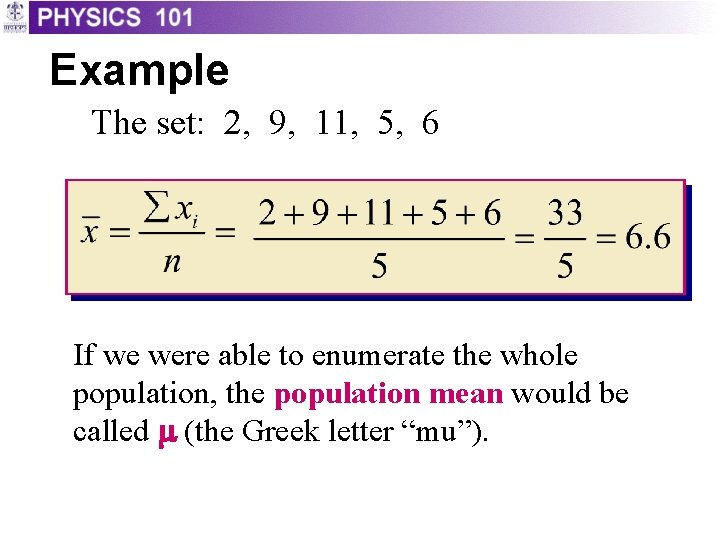
Example The set: 2, 9, 11, 5, 6 If we were able to enumerate the whole population, the population mean would be called m (the Greek letter “mu”).

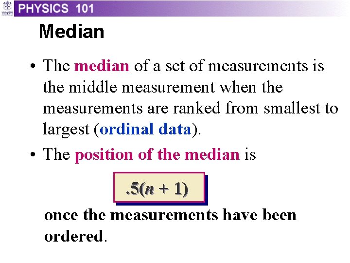
Median • The median of a set of measurements is the middle measurement when the measurements are ranked from smallest to largest (ordinal data). • The position of the median is. 5(n + 1) once the measurements have been ordered.

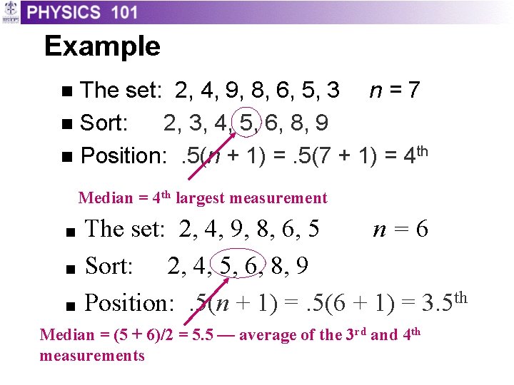
Example The set: 2, 4, 9, 8, 6, 5, 3 n = 7 n Sort: 2, 3, 4, 5, 6, 8, 9 n Position: . 5(n + 1) =. 5(7 + 1) = 4 th n Median = 4 th largest measurement The set: 2, 4, 9, 8, 6, 5 n=6 ■ Sort: 2, 4, 5, 6, 8, 9 ■ Position: . 5(n + 1) =. 5(6 + 1) = 3. 5 th ■ Median = (5 + 6)/2 = 5. 5 — average of the 3 rd and 4 th measurements

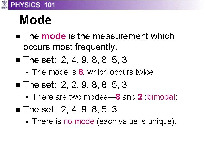
Mode The mode is the measurement which occurs most frequently. n The set: 2, 4, 9, 8, 8, 5, 3 n • n The set: 2, 2, 9, 8, 8, 5, 3 • n The mode is 8, which occurs twice There are two modes— 8 and 2 (bimodal) The set: 2, 4, 9, 8, 5, 3 • There is no mode (each value is unique).

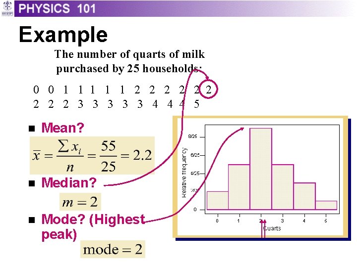
Example The number of quarts of milk purchased by 25 households: 0 0 1 1 1 2 2 2 2 2 3 3 3 4 4 4 5 n Mean? n Median? n Mode? (Highest peak)

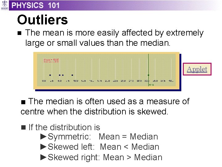
Outliers n The mean is more easily affected by extremely large or small values than the median. Applet ■ The median is often used as a measure of centre when the distribution is skewed. n If the distribution is ►Symmetric: Mean = Median ►Skewed left: Mean < Median ►Skewed right: Mean > Median

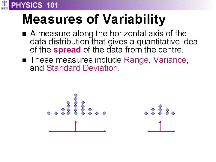
Measures of Variability n n A measure along the horizontal axis of the data distribution that gives a quantitative idea of the spread of the data from the centre. These measures include Range, Variance, and Standard Deviation.

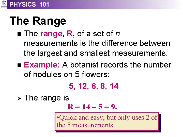
The Range The range, R, of a set of n measurements is the difference between the largest and smallest measurements. n Example: A botanist records the number of nodules on 5 flowers: 5, 12, 6, 8, 14 Ø The range is R = 14 – 5 = 9. n • Quick and easy, but only uses 2 of the 5 measurements.

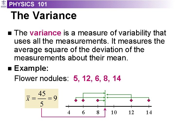
The Variance The variance is a measure of variability that uses all the measurements. It measures the average square of the deviation of the measurements about their mean. n Example: Flower nodules: 5, 12, 6, 8, 14 n 4 6 8 10 12 14

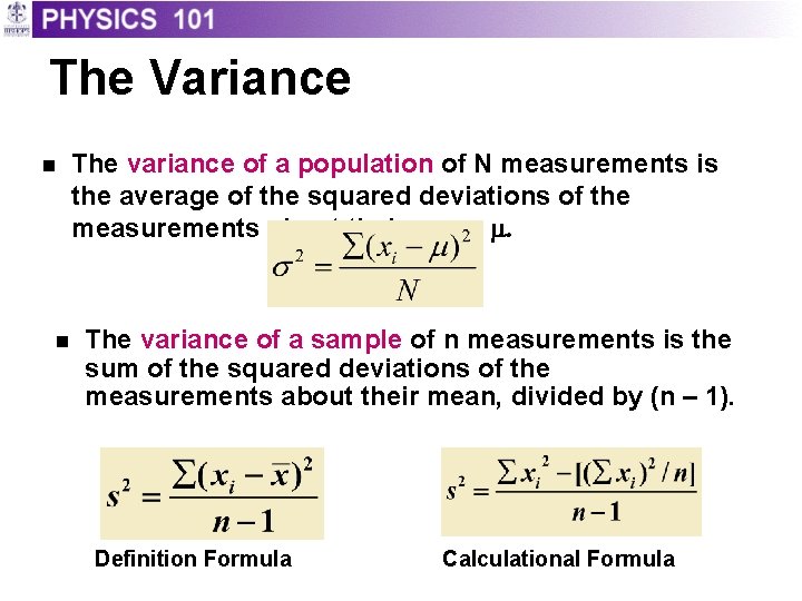
The Variance n n The variance of a population of N measurements is the average of the squared deviations of the measurements about their mean m. The variance of a sample of n measurements is the sum of the squared deviations of the measurements about their mean, divided by (n – 1). Definition Formula Calculational Formula

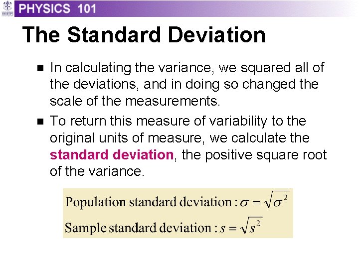
The Standard Deviation n n In calculating the variance, we squared all of the deviations, and in doing so changed the scale of the measurements. To return this measure of variability to the original units of measure, we calculate the standard deviation, the positive square root of the variance.

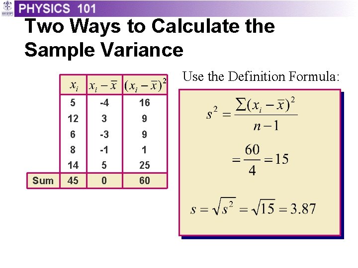
Two Ways to Calculate the Sample Variance Use the Definition Formula: Sum 5 -4 16 12 3 9 6 -3 9 8 -1 1 14 5 25 45 0 60

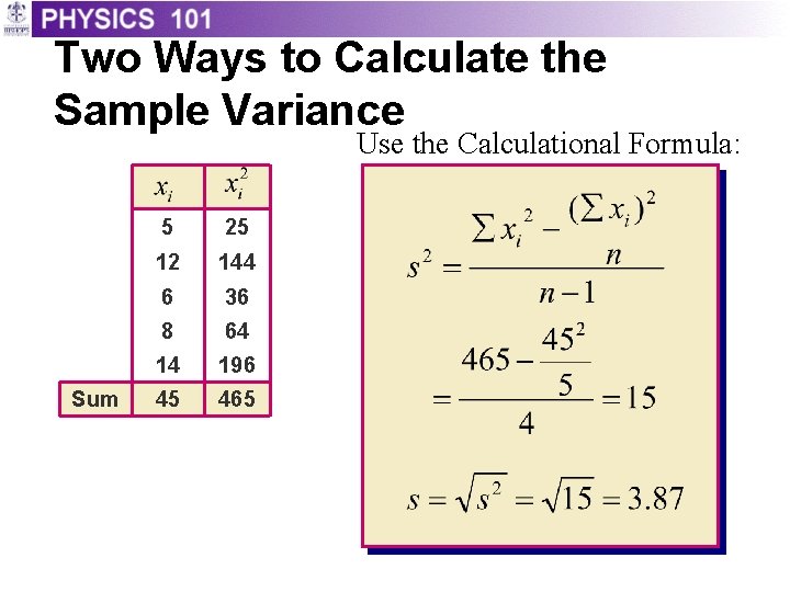
Two Ways to Calculate the Sample Variance Use the Calculational Formula: Sum 5 25 12 144 6 36 8 64 14 196 45 465

Some Notes The value of s is ALWAYS positive. n The larger the value of s, the larger the variability of the data set. Applet n Why divide by n – 1? n • The sample standard deviation s is often used to estimate the population standard deviation s. Dividing by n – 1 gives us a better estimate of s. Since the sample mean must be calculated first to obtain s, we say that the number of degrees of freedom has been reduced by one.

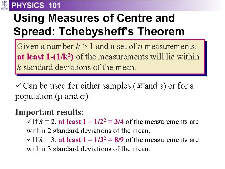
Using Measures of Centre and Spread: Tchebysheff’s Theorem Given a number k > 1 and a set of n measurements, at least 1 -(1/k 2) of the measurements will lie within k standard deviations of the mean. ü Can be used for either samples ( population (m and s) or for a Important results: üIf k = 2, at least 1 – 1/22 = 3/4 of the measurements are within 2 standard deviations of the mean. üIf k = 3, at least 1 – 1/32 = 8/9 of the measurements are within 3 standard deviations of the mean.

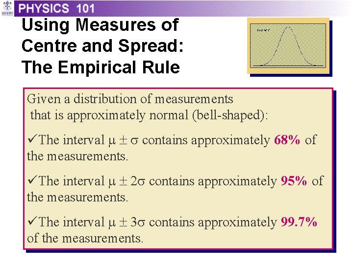
Using Measures of Centre and Spread: The Empirical Rule Given a distribution of measurements that is approximately normal (bell-shaped): üThe interval m s contains approximately 68% of the measurements. üThe interval m 2 s contains approximately 95% of the measurements. üThe interval m 3 s contains approximately 99. 7% of the measurements.

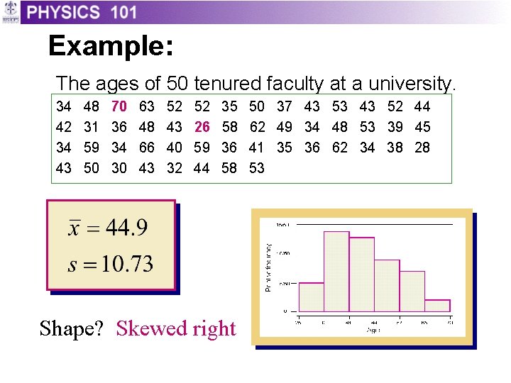
Example: The ages of 50 tenured faculty at a university. 34 42 34 43 48 31 59 50 70 36 34 30 63 48 66 43 52 43 40 32 52 26 59 44 35 58 36 58 Shape? Skewed right 50 37 43 53 43 52 44 62 49 34 48 53 39 45 41 35 36 62 34 38 28 53

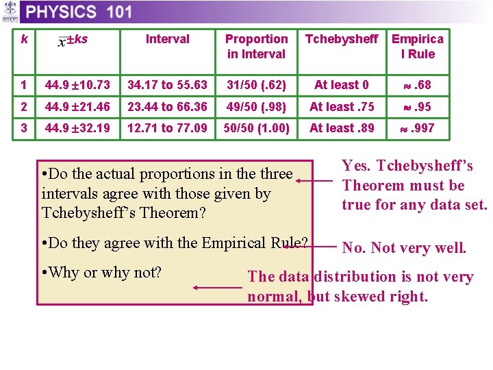
k ks Interval Proportion in Interval Tchebysheff Empirica l Rule 1 44. 9 10. 73 34. 17 to 55. 63 31/50 (. 62) At least 0 . 68 2 44. 9 21. 46 23. 44 to 66. 36 49/50 (. 98) At least. 75 . 95 3 44. 9 32. 19 12. 71 to 77. 09 50/50 (1. 00) At least. 89 . 997 • Do the actual proportions in the three intervals agree with those given by Tchebysheff’s Theorem? Yes. Tchebysheff’s Theorem must be true for any data set. • Do they agree with the Empirical Rule? No. Not very well. • Why or why not? The data distribution is not very normal, but skewed right.

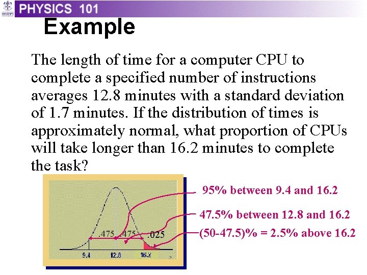
Example The length of time for a computer CPU to complete a specified number of instructions averages 12. 8 minutes with a standard deviation of 1. 7 minutes. If the distribution of times is approximately normal, what proportion of CPUs will take longer than 16. 2 minutes to complete the task? 95% between 9. 4 and 16. 2 47. 5% between 12. 8 and 16. 2. 475 . 025 (50 -47. 5)% = 2. 5% above 16. 2

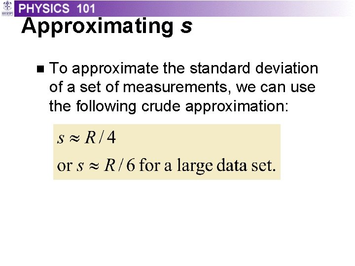
Approximating s n To approximate the standard deviation of a set of measurements, we can use the following crude approximation:

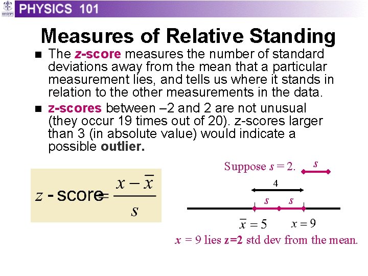
Measures of Relative Standing n n The z-score measures the number of standard deviations away from the mean that a particular measurement lies, and tells us where it stands in relation to the other measurements in the data. z-scores between – 2 and 2 are not unusual (they occur 19 times out of 20). z-scores larger than 3 (in absolute value) would indicate a possible outlier. Suppose s = 2. s 4 s s x = 9 lies z=2 std dev from the mean.

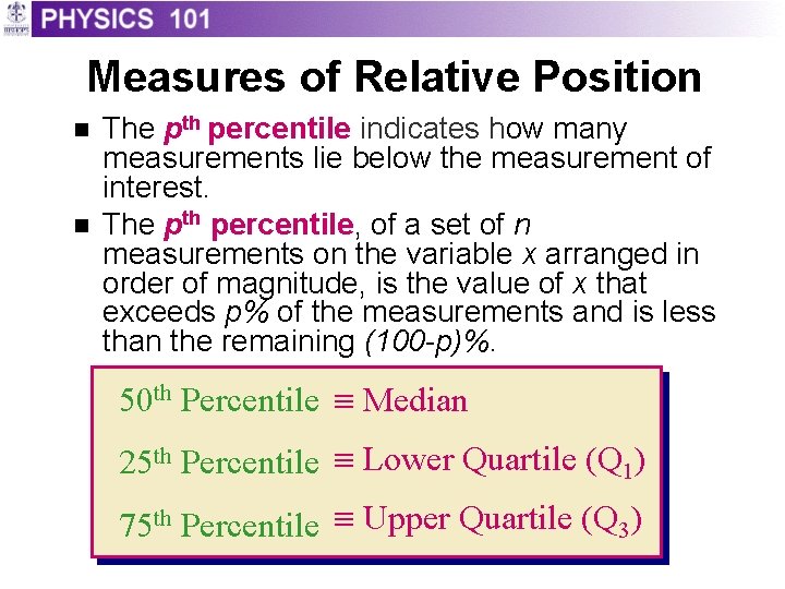
Measures of Relative Position n n The pth percentile indicates how many measurements lie below the measurement of interest. The pth percentile, of a set of n measurements on the variable x arranged in order of magnitude, is the value of x that exceeds p% of the measurements and is less than the remaining (100 -p)%. 50 th Percentile Median 25 th Percentile Lower Quartile (Q 1) 75 th Percentile Upper Quartile (Q 3)

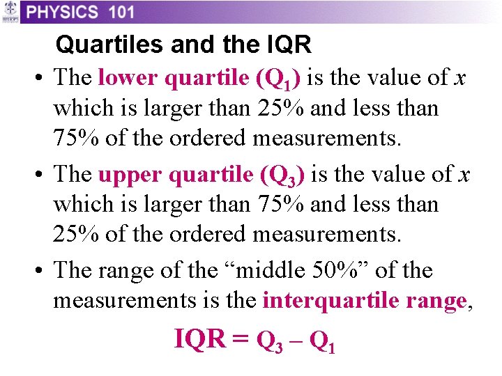
Quartiles and the IQR • The lower quartile (Q 1) is the value of x which is larger than 25% and less than 75% of the ordered measurements. • The upper quartile (Q 3) is the value of x which is larger than 75% and less than 25% of the ordered measurements. • The range of the “middle 50%” of the measurements is the interquartile range, IQR = Q 3 – Q 1

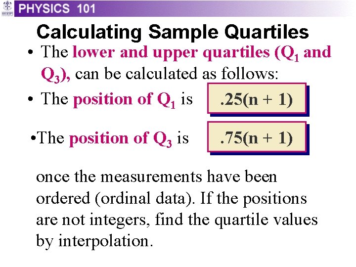
Calculating Sample Quartiles • The lower and upper quartiles (Q 1 and Q 3), can be calculated as follows: • The position of Q 1 is. 25(n + 1) • The position of Q 3 is . 75(n + 1) once the measurements have been ordered (ordinal data). If the positions are not integers, find the quartile values by interpolation.

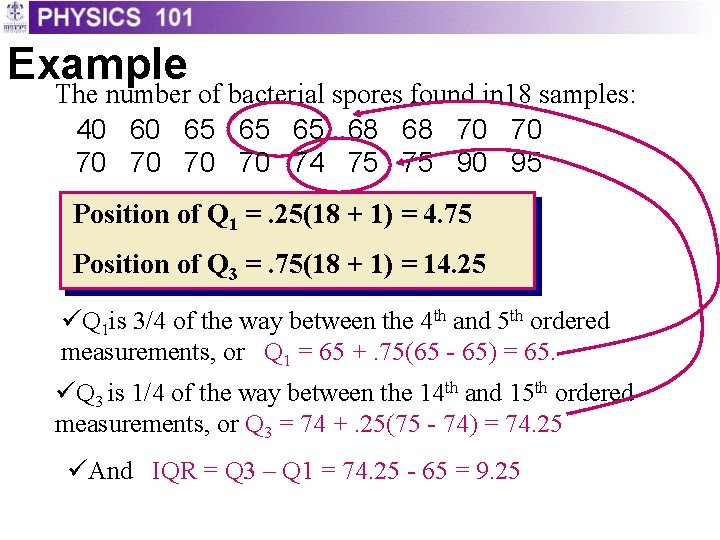
Example The number of bacterial spores found in 18 samples: 40 60 65 65 65 68 68 70 70 70 74 75 75 90 95 Position of Q 1 =. 25(18 + 1) = 4. 75 Position of Q 3 =. 75(18 + 1) = 14. 25 üQ 1 is 3/4 of the way between the 4 th and 5 th ordered measurements, or Q 1 = 65 +. 75(65 - 65) = 65. üQ 3 is 1/4 of the way between the 14 th and 15 th ordered measurements, or Q 3 = 74 +. 25(75 - 74) = 74. 25 üAnd IQR = Q 3 – Q 1 = 74. 25 - 65 = 9. 25

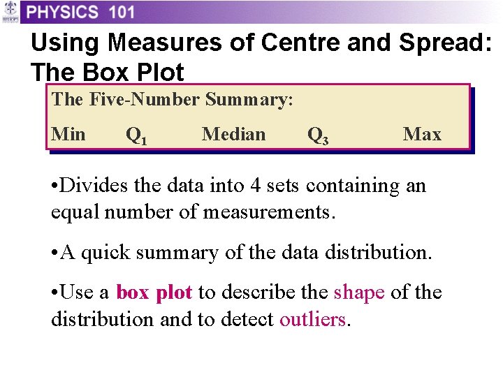
Using Measures of Centre and Spread: The Box Plot The Five-Number Summary: Min Q 1 Median Q 3 Max • Divides the data into 4 sets containing an equal number of measurements. • A quick summary of the data distribution. • Use a box plot to describe the shape of the distribution and to detect outliers.

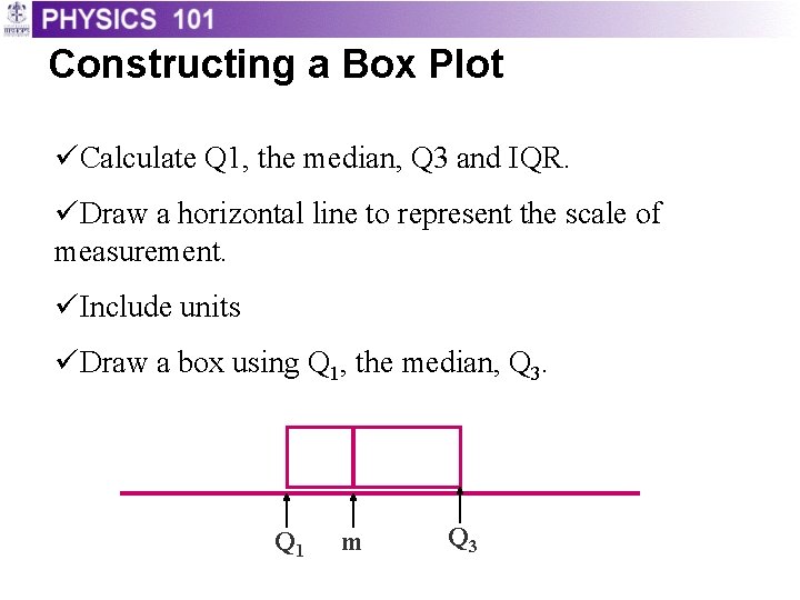
Constructing a Box Plot üCalculate Q 1, the median, Q 3 and IQR. üDraw a horizontal line to represent the scale of measurement. üInclude units üDraw a box using Q 1, the median, Q 3. Q 1 m Q 3

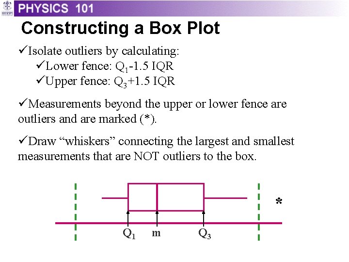
Constructing a Box Plot üIsolate outliers by calculating: üLower fence: Q 1 -1. 5 IQR üUpper fence: Q 3+1. 5 IQR üMeasurements beyond the upper or lower fence are outliers and are marked (*). üDraw “whiskers” connecting the largest and smallest measurements that are NOT outliers to the box. * Q 1 m Q 3

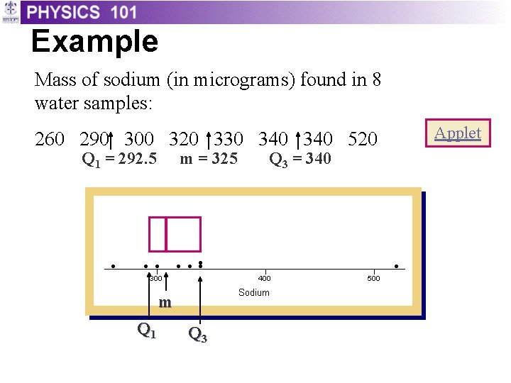
Example Mass of sodium (in micrograms) found in 8 water samples: 260 290 300 320 330 340 520 Q 1 = 292. 5 m = 325 m Q 1 Q 3 = 340 Applet

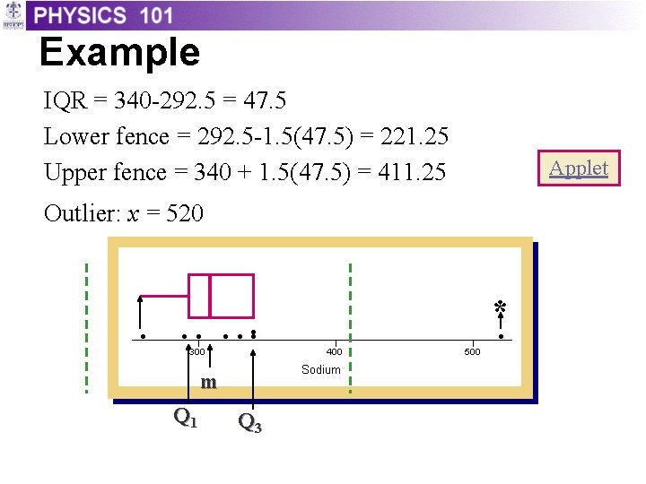
Example IQR = 340 -292. 5 = 47. 5 Lower fence = 292. 5 -1. 5(47. 5) = 221. 25 Upper fence = 340 + 1. 5(47. 5) = 411. 25 Applet Outlier: x = 520 * m Q 1 Q 3

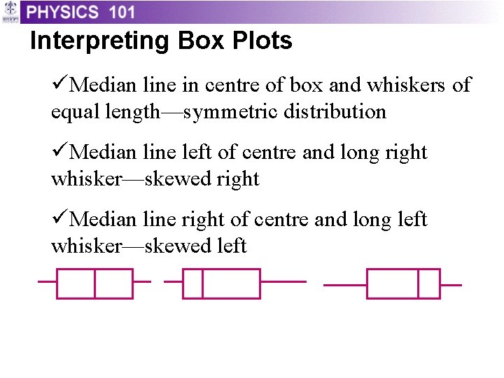
Interpreting Box Plots üMedian line in centre of box and whiskers of equal length—symmetric distribution üMedian line left of centre and long right whisker—skewed right üMedian line right of centre and long left whisker—skewed left

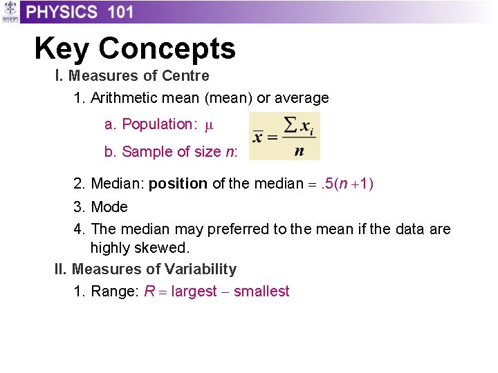
Key Concepts I. Measures of Centre 1. Arithmetic mean (mean) or average a. Population: m b. Sample of size n: 2. Median: position of the median =. 5(n +1) 3. Mode 4. The median may preferred to the mean if the data are highly skewed. II. Measures of Variability 1. Range: R = largest - smallest

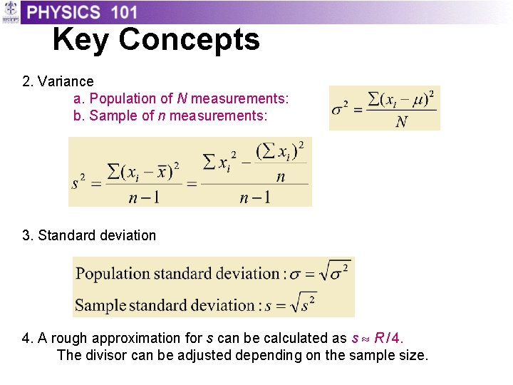
Key Concepts 2. Variance a. Population of N measurements: b. Sample of n measurements: 3. Standard deviation 4. A rough approximation for s can be calculated as s » R / 4. The divisor can be adjusted depending on the sample size.

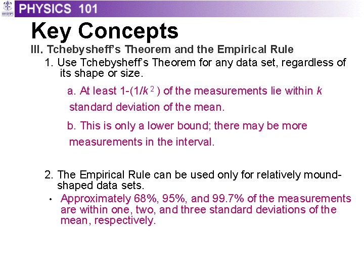
Key Concepts III. Tchebysheff’s Theorem and the Empirical Rule 1. Use Tchebysheff’s Theorem for any data set, regardless of its shape or size. a. At least 1 -(1/k 2 ) of the measurements lie within k standard deviation of the mean. b. This is only a lower bound; there may be more measurements in the interval. 2. The Empirical Rule can be used only for relatively moundshaped data sets. • Approximately 68%, 95%, and 99. 7% of the measurements are within one, two, and three standard deviations of the mean, respectively.

Key Concepts IV. Measures of Relative Standing 1. Sample z-score: 2. pth percentile; p% of the measurements are smaller, and (100 - p)% are larger. 3. Lower quartile, Q 1; position of Q 1 =. 25(n +1) 4. Upper quartile, Q 3 ; position of Q 3 =. 75(n +1) 5. Interquartile range: IQR = Q 3 - Q 1 V. Box Plots 1. Box plots are used for detecting outliers and shapes of distributions. 2. Q 1 and Q 3 form the ends of the box. The median line is in the interior of the box.

Key Concepts 3. Upper and lower fences are used to find outliers. a. Lower fence: Q 1 - 1. 5(IQR) b. Outer fences: Q 3 + 1. 5(IQR) 4. Whiskers are connected to the smallest and largest measurements that are not outliers. 5. Skewed distributions usually have a long whisker in the direction of the skewness, and the median line is drawn away from the direction of the skewness.