Chapter 2 Demand Supply Market Equilibrium 2016 by

Chapter 2 Demand, Supply, & Market Equilibrium © 2016 by Mc. Graw-Hill Education. This is proprietary material solely for authorized instructor use. Not authorized for sale or distribution in any manner. This document may not be copied, scanned, duplicated, forwarded, distributed, or posted on a website, in whole or part. 1 -1

Learning Objectives v Identify demand functions and distinguish between a change in demand a change in quantity demanded v Identify supply functions and distinguish between a change in supply and a change in quantity supplied v Explain why market equilibrium occurs at the price for which quantity demanded equals quantity supplied v Measure gains from market exchange using consumer surplus, producer surplus, and social surplus v Predict the impact on equilibrium price and quantity of shifts in demand or supply v Examine the impact of government imposed price ceilings and price floors © 2016 by Mc. Graw-Hill Education. This is proprietary material solely for authorized instructor use. Not authorized for sale or distribution in any manner. This document may not be copied, scanned, duplicated, forwarded, distributed, or posted on a website, in whole or part. 2 -2

Demand v Quantity demanded (Qd) ~ Amount of a good or service consumers are willing & able to purchase during a given period of time © 2016 by Mc. Graw-Hill Education. This is proprietary material solely for authorized instructor use. Not authorized for sale or distribution in any manner. This document may not be copied, scanned, duplicated, forwarded, distributed, or posted on a website, in whole or part. 2 -3

General Demand Function v Six variables that influence Qd ~ Price of good or service (P) ~ Incomes of consumers (M) ~ Prices of related goods & services (PR) ~ Taste patterns of consumers (T) ~ Expected future price of product (PE) ~ Number of consumers in market (N) v General demand function Qd = f(P, M, PR, T, PE , N) © 2016 by Mc. Graw-Hill Education. This is proprietary material solely for authorized instructor use. Not authorized for sale or distribution in any manner. This document may not be copied, scanned, duplicated, forwarded, distributed, or posted on a website, in whole or part. 2 -4

General Demand Function Qd = a + b. P + c. M + d. PR + e. T + f. PE + g. N v b, c, d, e, f, & g are slope parameters ~ Measure effect on Qd of changing one of the variables while holding the others constant v Sign of parameter shows how variable is related to Qd ~ Positive sign indicates direct relationship ~ Negative sign indicates inverse relationship © 2016 by Mc. Graw-Hill Education. This is proprietary material solely for authorized instructor use. Not authorized for sale or distribution in any manner. This document may not be copied, scanned, duplicated, forwarded, distributed, or posted on a website, in whole or part. 2 -5

General Demand Function v Normal good ~ A good or service for which an increase (decrease) in income causes consumers to demand more (less) of the good, holding all other variables in the general demand function constant v Inferior good ~ A good or service for which an increase (decrease) in income causes consumers to demand less (more) of the good, all other factors held constant © 2016 by Mc. Graw-Hill Education. This is proprietary material solely for authorized instructor use. Not authorized for sale or distribution in any manner. This document may not be copied, scanned, duplicated, forwarded, distributed, or posted on a website, in whole or part. 2 -6

General Demand Function v Substitutes ~ Two goods are substitutes if an increase (decrease) in the price of one good causes consumers to demand more (less) of the other good, holding all other factors constant v Complements ~ Two goods are complements if an increase (decrease) in the price of one good causes consumers to demand less (more) of the other good, all other things held constant © 2016 by Mc. Graw-Hill Education. This is proprietary material solely for authorized instructor use. Not authorized for sale or distribution in any manner. This document may not be copied, scanned, duplicated, forwarded, distributed, or posted on a website, in whole or part. 2 -7

General Demand Function Variable Relation to Qd P Inverse M Direct for normal goods Inverse for inferior goods PR Sign of Slope Parameter b = Qd/ P is negative c = Qd/ M is positive c = Qd/ M is negative d = Qd/ PR is positive Direct for substitutes Inverse for complements d = Qd/ PR is negative T Direct e = Qd/ T is positive PE Direct f = Qd/ PE is positive N Direct g = Qd/ N is positive © 2016 by Mc. Graw-Hill Education. This is proprietary material solely for authorized instructor use. Not authorized for sale or distribution in any manner. This document may not be copied, scanned, duplicated, forwarded, distributed, or posted on a website, in whole or part. 2 -8

Direct Demand Function v The direct demand function, or simply demand, shows how quantity demanded, Qd , is related to product price, P, when all other variables are held constant ~ Qd = f(P) v Law of Demand ~ Qd increases when P falls, all else constant ~ Qd decreases when P rises, all else constant ~ Qd/ P must be negative © 2016 by Mc. Graw-Hill Education. This is proprietary material solely for authorized instructor use. Not authorized for sale or distribution in any manner. This document may not be copied, scanned, duplicated, forwarded, distributed, or posted on a website, in whole or part. 2 -9

Inverse Demand Function v Traditionally, price (P) is plotted on the vertical axis & quantity demanded (Qd) is plotted on the horizontal axis ~ The equation plotted is the inverse demand function, P = f(Qd) © 2016 by Mc. Graw-Hill Education. This is proprietary material solely for authorized instructor use. Not authorized for sale or distribution in any manner. This document may not be copied, scanned, duplicated, forwarded, distributed, or posted on a website, in whole or part. 2 -10

Graphing Demand Curves v A point on a direct demand curve shows either: ~ Maximum amount of a good that will be purchased for a given price ~ Maximum price consumers will pay for a specific amount of the good (demand price) © 2016 by Mc. Graw-Hill Education. This is proprietary material solely for authorized instructor use. Not authorized for sale or distribution in any manner. This document may not be copied, scanned, duplicated, forwarded, distributed, or posted on a website, in whole or part. 2 -11

A Demand Curve (Figure 2. 1) Qd = 1, 400 – 10 P © 2016 by Mc. Graw-Hill Education. This is proprietary material solely for authorized instructor use. Not authorized for sale or distribution in any manner. This document may not be copied, scanned, duplicated, forwarded, distributed, or posted on a website, in whole or part. 2 -12

Graphing Demand Curves v Change in quantity demanded ~ Occurs when price changes ~ Movement along demand curve v Change in demand ~ Occurs when one of the other variables, or determinants of demand, changes ~ Demand curve shifts rightward or leftward © 2016 by Mc. Graw-Hill Education. This is proprietary material solely for authorized instructor use. Not authorized for sale or distribution in any manner. This document may not be copied, scanned, duplicated, forwarded, distributed, or posted on a website, in whole or part. 2 -13

Shifts in Demand (Figure 2. 2) © 2016 by Mc. Graw-Hill Education. This is proprietary material solely for authorized instructor use. Not authorized for sale or distribution in any manner. This document may not be copied, scanned, duplicated, forwarded, distributed, or posted on a website, in whole or part. 2 -14

Supply v Quantity supplied (Qs) ~ Amount of a good or service offered for sale during a given period of time © 2016 by Mc. Graw-Hill Education. This is proprietary material solely for authorized instructor use. Not authorized for sale or distribution in any manner. This document may not be copied, scanned, duplicated, forwarded, distributed, or posted on a website, in whole or part. 2 -15

Supply v Six variables that influence Qs ~ Price of good or service (P) ~ Input prices (PI ) ~ Prices of goods related in production (Pr) ~ Technological advances (T) ~ Expected future price of product (Pe) ~ Number of firms producing product (F) v General supply function Qs = f(P, PI, Pr, T, Pe, F) © 2016 by Mc. Graw-Hill Education. This is proprietary material solely for authorized instructor use. Not authorized for sale or distribution in any manner. This document may not be copied, scanned, duplicated, forwarded, distributed, or posted on a website, in whole or part. 2 -16

General Supply Function Qs = h + k. P + l. PI + m. Pr + n. T + r. Pe + s. F v k, l, m, n, r, & s are slope parameters ~ Measure effect on Qs of changing one of the variables while holding the others constant v Sign of parameter shows how variable is related to Qs ~ Positive sign indicates direct relationship ~ Negative sign indicates inverse relationship © 2016 by Mc. Graw-Hill Education. This is proprietary material solely for authorized instructor use. Not authorized for sale or distribution in any manner. This document may not be copied, scanned, duplicated, forwarded, distributed, or posted on a website, in whole or part. 2 -17

General Supply Function v Substitutes in production ~ Goods for which an increase in the price of one good relative to the price of another good causes producers to increase production of the now higher-priced good and decrease production of the other good v Complements in production ~ Goods for which an increase in the price of one good, relative to the price of another good, causes producers to increase production of both goods © 2016 by Mc. Graw-Hill Education. This is proprietary material solely for authorized instructor use. Not authorized for sale or distribution in any manner. This document may not be copied, scanned, duplicated, forwarded, distributed, or posted on a website, in whole or part. 2 -18

General Supply Function Variable Relation to Qs Sign of Slope Parameter P Direct k = Qs/ P is positive PI Inverse l = Qs/ PI is negative Pr Inverse for substitutes Direct for complements m = Qs/ Pr is negative m = Qs/ Pr is positive T Direct n = Qs/ T is positive Pe Inverse r = Qs/ Pe is negative F Direct s = Qs/ F is positive © 2016 by Mc. Graw-Hill Education. This is proprietary material solely for authorized instructor use. Not authorized for sale or distribution in any manner. This document may not be copied, scanned, duplicated, forwarded, distributed, or posted on a website, in whole or part. 2 -19

Direct Supply Function v The direct supply function, or simply supply, shows how quantity supplied, Qs , is related to product price, P, when all other variables are held constant ~ Qs = f(P) © 2016 by Mc. Graw-Hill Education. This is proprietary material solely for authorized instructor use. Not authorized for sale or distribution in any manner. This document may not be copied, scanned, duplicated, forwarded, distributed, or posted on a website, in whole or part. 2 -20

Inverse Supply Function v Traditionally, price (P) is plotted on the vertical axis & quantity supplied (Qs) is plotted on the horizontal axis ~ The equation plotted is the inverse supply function, P = f(Qs) © 2016 by Mc. Graw-Hill Education. This is proprietary material solely for authorized instructor use. Not authorized for sale or distribution in any manner. This document may not be copied, scanned, duplicated, forwarded, distributed, or posted on a website, in whole or part. 2 -21

Graphing Supply Curves v A point on a direct supply curve shows either: ~ Maximum amount of a good that will be offered for sale at a given price ~ Minimum price necessary to induce producers to voluntarily offer a given quantity for sale (supply price) © 2016 by Mc. Graw-Hill Education. This is proprietary material solely for authorized instructor use. Not authorized for sale or distribution in any manner. This document may not be copied, scanned, duplicated, forwarded, distributed, or posted on a website, in whole or part. 2 -22

A Supply Curve (Figure 2. 3) Qs = -400 + 20 P © 2016 by Mc. Graw-Hill Education. This is proprietary material solely for authorized instructor use. Not authorized for sale or distribution in any manner. This document may not be copied, scanned, duplicated, forwarded, distributed, or posted on a website, in whole or part. 2 -23

Graphing Supply Curves v Change in quantity supplied ~ Occurs when price changes ~ Movement along supply curve v Change in supply ~ Occurs when one of the other variables, or determinants of supply, changes ~ Supply curve shifts rightward or leftward © 2016 by Mc. Graw-Hill Education. This is proprietary material solely for authorized instructor use. Not authorized for sale or distribution in any manner. This document may not be copied, scanned, duplicated, forwarded, distributed, or posted on a website, in whole or part. 2 -24

Shifts in Supply (Figure 2. 4) © 2016 by Mc. Graw-Hill Education. This is proprietary material solely for authorized instructor use. Not authorized for sale or distribution in any manner. This document may not be copied, scanned, duplicated, forwarded, distributed, or posted on a website, in whole or part. 2 -25

Market Equilibrium v Equilibrium price & quantity are determined by the intersection of demand & supply curves ~ At the point of intersection, Qd = Qs ~ Consumers can purchase all they want & producers can sell all they want at the “market-clearing” or “equilibrium” price © 2016 by Mc. Graw-Hill Education. This is proprietary material solely for authorized instructor use. Not authorized for sale or distribution in any manner. This document may not be copied, scanned, duplicated, forwarded, distributed, or posted on a website, in whole or part. 2 -26

Market Equilibrium (Figure 2. 5) © 2016 by Mc. Graw-Hill Education. This is proprietary material solely for authorized instructor use. Not authorized for sale or distribution in any manner. This document may not be copied, scanned, duplicated, forwarded, distributed, or posted on a website, in whole or part. 2 -27

Market Equilibrium v Excess supply (surplus) ~ Exists when quantity supplied exceeds quantity demanded v Excess demand (shortage) ~ Exists when quantity demanded exceeds quantity supplied © 2016 by Mc. Graw-Hill Education. This is proprietary material solely for authorized instructor use. Not authorized for sale or distribution in any manner. This document may not be copied, scanned, duplicated, forwarded, distributed, or posted on a website, in whole or part. 2 -28

Value of Market Exchange v Typically, consumers value the goods they purchase by an amount that exceeds the purchase price of the goods v Economic value ~ Maximum amount any buyer in the market is willing to pay for the unit, which is measured by the demand price for the unit of the good © 2016 by Mc. Graw-Hill Education. This is proprietary material solely for authorized instructor use. Not authorized for sale or distribution in any manner. This document may not be copied, scanned, duplicated, forwarded, distributed, or posted on a website, in whole or part. 2 -29

Measuring the Value of Market Exchange v Consumer surplus ~ Difference between the economic value of a good (its demand price) & the market price the consumer must pay v Producer surplus ~ For each unit supplied, difference between market price & the minimum price producers would accept to supply the unit (its supply price) v Social surplus ~ Sum of consumer & producer surplus ~ Area below demand & above supply over the relevant range of output © 2016 by Mc. Graw-Hill Education. This is proprietary material solely for authorized instructor use. Not authorized for sale or distribution in any manner. This document may not be copied, scanned, duplicated, forwarded, distributed, or posted on a website, in whole or part. 2 -30

Measuring the Value of Market Exchange (Figure 2. 6) © 2016 by Mc. Graw-Hill Education. This is proprietary material solely for authorized instructor use. Not authorized for sale or distribution in any manner. This document may not be copied, scanned, duplicated, forwarded, distributed, or posted on a website, in whole or part. 2 -31

Changes in Market Equilibrium v Qualitative forecast ~ Predicts only the direction in which an economic variable will move v Quantitative forecast ~ Predicts both the direction and the magnitude of the change in an economic variable © 2016 by Mc. Graw-Hill Education. This is proprietary material solely for authorized instructor use. Not authorized for sale or distribution in any manner. This document may not be copied, scanned, duplicated, forwarded, distributed, or posted on a website, in whole or part. 2 -32

Demand Shifts (Supply Constant) (Figure 2. 7) © 2016 by Mc. Graw-Hill Education. This is proprietary material solely for authorized instructor use. Not authorized for sale or distribution in any manner. This document may not be copied, scanned, duplicated, forwarded, distributed, or posted on a website, in whole or part. 2 -33

Supply Shifts (Demand Constant) (Figure 2. 8) © 2016 by Mc. Graw-Hill Education. This is proprietary material solely for authorized instructor use. Not authorized for sale or distribution in any manner. This document may not be copied, scanned, duplicated, forwarded, distributed, or posted on a website, in whole or part. 2 -34

Simultaneous Shifts v When demand & supply shift simultaneously ~ Can predict either the direction in which price changes or the direction in which quantity changes, but not both ~ The change in equilibrium price or quantity is said to be indeterminate when the direction of change depends on the relative magnitudes by which demand & supply shift © 2016 by Mc. Graw-Hill Education. This is proprietary material solely for authorized instructor use. Not authorized for sale or distribution in any manner. This document may not be copied, scanned, duplicated, forwarded, distributed, or posted on a website, in whole or part. 2 -35

Simultaneous Shifts: ( D, S) P S S′ S′′ B P′ P P′′ • A • • C D′ D Q Q Q′ Q′′ Price may rise or fall; Quantity rises © 2016 by Mc. Graw-Hill Education. This is proprietary material solely for authorized instructor use. Not authorized for sale or distribution in any manner. This document may not be copied, scanned, duplicated, forwarded, distributed, or posted on a website, in whole or part. 2 -36

Simultaneous Shifts: ( D, S) P S S′ S′ A • P P′ P′′ • B • C D D′ Q Q′′ Price falls; Quantity may rise or fall © 2016 by Mc. Graw-Hill Education. This is proprietary material solely for authorized instructor use. Not authorized for sale or distribution in any manner. This document may not be copied, scanned, duplicated, forwarded, distributed, or posted on a website, in whole or part. 2 -37

Simultaneous Shifts: ( D, S) P S′′ S′ P′′ • C • P′ S B A • P D′ D Q Q′′ Q Q′ Price rises; Quantity may rise or fall © 2016 by Mc. Graw-Hill Education. This is proprietary material solely for authorized instructor use. Not authorized for sale or distribution in any manner. This document may not be copied, scanned, duplicated, forwarded, distributed, or posted on a website, in whole or part. 2 -38

Simultaneous Shifts: ( D, S) P S′′ P P′ • C • S′ S A B • D D′ Q′ Q Q Price may rise or fall; Quantity falls © 2016 by Mc. Graw-Hill Education. This is proprietary material solely for authorized instructor use. Not authorized for sale or distribution in any manner. This document may not be copied, scanned, duplicated, forwarded, distributed, or posted on a website, in whole or part. 2 -39

Ceiling & Floor Prices v Ceiling price ~ Maximum price government permits sellers to charge for a good ~ When ceiling price is below equilibrium, a shortage occurs v Floor price ~ Minimum price government permits sellers to charge for a good ~ When floor price is above equilibrium, a surplus occurs © 2016 by Mc. Graw-Hill Education. This is proprietary material solely for authorized instructor use. Not authorized for sale or distribution in any manner. This document may not be copied, scanned, duplicated, forwarded, distributed, or posted on a website, in whole or part. 2 -40

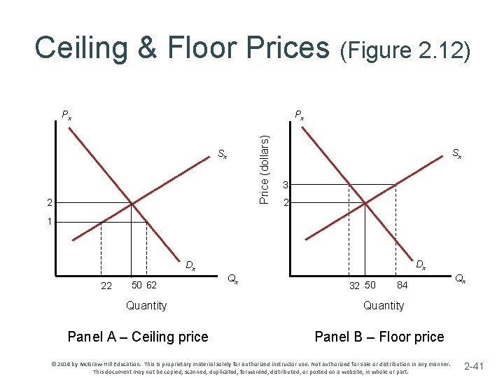
Ceiling & Floor Prices (Figure 2. 12) Px Price (dollars) Px Sx 2 Sx 3 2 1 Dx Dx 22 50 62 Quantity Panel A – Ceiling price Qx 32 50 84 Qx Quantity Panel B – Floor price © 2016 by Mc. Graw-Hill Education. This is proprietary material solely for authorized instructor use. Not authorized for sale or distribution in any manner. This document may not be copied, scanned, duplicated, forwarded, distributed, or posted on a website, in whole or part. 2 -41

Summary v 6 variables influence demand: good’s price, income, prices of related goods, consumers’ tastes, expected future price, and number of consumers ~ Law of demand states that quantity demanded increases (decreases) when price falls (rises), all else constant v 6 variables influence supply: good’s price, input prices, prices of goods related in production, producers’ expectation of future price, number of firms v Equilibrium price and quantity determined by intersection of supply and demand curves v Consumer surplus arises because the equilibrium price consumers pay is less than the value they place on the units they purchase. © 2016 by Mc. Graw-Hill Education. This is proprietary material solely for authorized instructor use. Not authorized for sale or distribution in any manner. This document may not be copied, scanned, duplicated, forwarded, distributed, or posted on a website, in whole or part. 2 -42

Summary v Consumer surplus arises because the equilibrium price consumers pay is less than the value they place on units they purchase ~ Producer surplus arises because equilibrium price is greater than the minimum price producers would be willing to accept to produce. ~ Social surplus: sum of consumer surplus and producer surplus v When both supply and demand shift simultaneously, one can predict either the direction of change in price or the direction of change in quantity, but not both v A ceiling price (below equilibrium) results in a shortage; a floor price (above equilibrium) results in a surplus © 2016 by Mc. Graw-Hill Education. This is proprietary material solely for authorized instructor use. Not authorized for sale or distribution in any manner. This document may not be copied, scanned, duplicated, forwarded, distributed, or posted on a website, in whole or part. 2 -43