Chapter 2 Appointment scheduling Plan Basis of Appointment

Chapter 2 Appointment scheduling

Plan • Basis of Appointment Systems • Individual-block/Variable-interval rule • Variable-block/Fixed-interval rule • A static appointment model with dynamic features • Managing the Appointments with Waiting Time Targets and Random Walk-ins - 2 -

Intoduction • Rising healthcare expenditure and increasing demand lead a growing pressure on health service providers to improve efficiency. • Appointment scheduling systems lie at the intersection of efficiency and timely access to health services. • Timely access is important for realizing good medical outcomes. It is also an important determinant of patient satisfaction. • The ability to provide timely access is determined by a variety of factors including both strategy designs (location, capacity, size) and operation management. • The issue of capacity planning is addressed in another chapter and an example of resource allocation in multisite service systems can be found in Chao et al. Chao, X. , Liu, L. and Zheng, S. (2003) Resource allocation in multisite service systems with intersite customer flows. Management Science, 49(12), 1739– 1752 - 3 -

Dimensions of appointment systems Goal : to find an Appointment System (AS) for which a particular measure of performance is optimized in a clinical environment—an application of resource scheduling under uncertainty. • Nature of decision-making • Modeling clinic environments • Mesures of performance • Appointment system design • Analysis methods T. Cayiri & E. Veral, « Outpatient scheduling in health care : a review of literature , » Production and Operations Management, 12/4, 2003 - 4 -

Nature of decision making Static vs dynamic appointment scheduling systems Static systems : • all decisions must be made prior to the beginning of a clinic session (day or half-day), which is the most common appointment system. • Most of the literature concentrates on the static problem. Dynamic case : • the schedule of future arrivals revised continuously over the course of the day based on the current state of the system • Applicable when patient arrivals can be regulated dynamically, which involves patients already admitted to a hospital or clinic. ? ? ? Possible with on-line apps? - 5 -

Modelling clinic environment Regarded as a queuing system characterized by the followings: • Number of services (single or multi-stage) • Number of doctors (single or multi-server) • Number of appointments per clinic session • Arrival process (deterministic or stochastic) • Punctuality of patients • Presence of no-shows • Presence of regular & emergency walk-ins (preemtive or not) • Presence of companions • Service times (empirical or theoretical distribution) • Lateness and interrruption of doctors • Queue discipline - 6 -

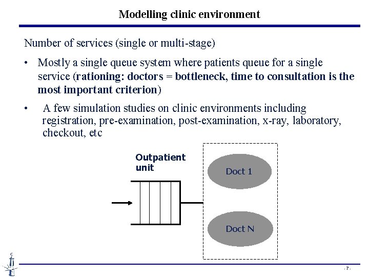
Modelling clinic environment Number of services (single or multi-stage) • Mostly a single queue system where patients queue for a single service (rationing: doctors = bottleneck, time to consultation is the most important criterion) • A few simulation studies on clinic environments including registration, pre-examination, post-examination, x-ray, laboratory, checkout, etc Outpatient unit Doct 1 Doct N - 7 -

Modelling clinic environment Number of doctors (servers) • Mostly a single server • Doctors have their own waiting list • Although pooling improves waiting times & utilisation, random doctor assignment is undesirable due to the desirable one-to-one doctor-patient relationship • Sending patients to the first available doctor is however practiced in some countries Warning : Multi-server setting is however realistic for diagnostic equipment (IMR, CT, …) - 8 -

Modelling clinic environment Number of Appointments per Clinic Session • There exists a positive relationship between waiting times and the number of appointments in a clinic session (N). • the effect of N is mitigated by no-shows and variability of consultation times, and thus cannot be easily generalized - 9 -

Modelling clinic environment The arrival process Unpunctuality of patients: • Empirical evidence : early more often than late. • patient earliness may also be undesirable, since it creates excessive congestion in the waiting area Presence of no-shows: • Empirical evidence : 5 -30% (even 40%) no-shows depending on the specialties. • Numerical observation : no-show proba is a major factor affecting the performance and the choice of AS • Depending on different variables (such as age, socioeconomic level, etc. ) • Countermeasures: overbooking but also mechanism to discouraging no-shows (blacklist? ) - 10 -

Modelling clinic environment The arrival process Unpunctuality of patients: Presence of no-shows: Presence of walk-ins (regular and emergency): • Rarely in UK hospital clinics used mainly for referred patients • But must be anticipated and planned for in some US clinics that are patient’s GP and respeonsible for patient’s total care, whether emergent or not. • Common in Chinese hospitals providing on-line appointment • Observation : walk-in varying across specialties and throughout the day, but not from day to day Presence of companions • Importan for waiting room area design Balking or reneging behavior - 11 -

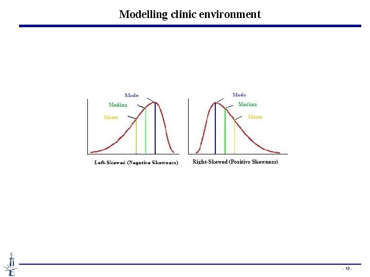
Modelling clinic environment Service times • sum of all the times a patient is claiming the doctor’s attention • Common model: homogenuous patients with iid service times independent of the arrival process (no response to congestion) • Empirical data: unimodal and right-skewed, CV = 0. 35 – 0. 85 • Erlang or exponential distribution in analytical studies • Observation 1: optimal solutions mostly dependent on mean and variance • Observation 2: high variability of service times deteriorates both patient wait and doctor’s idle time • Observation 3: shorter mean service time -> lower waiting time. • Technologies help reducing the consultation time - 12 -

Modelling clinic environment - 13 -

Modelling clinic environment Lateness and Interruption Level of Doctors • Agreement among existing studies is that patient waiting times are highly sensitive to this factor. • If the doctor does not start the clinic on time, a delay factor builds up from the start that ripples throughout the clinic session. • Another doctor-related factor is the interruption level (also called the “gap times”). • Game theory may be useful in modeling patient and doctor arrivals by considering the conflicting interests of both parties. • patients arrive late knowing that they will have to wait. • doctors may arrive late, being afraid that the first patient will be late. - 14 -

Modelling clinic environment Queueing discipline • Common model: FIFO • Reasonable for puctual patients • Unrealistic in the presence of unpunctuality as doctors would not keep idle waiting for the next appointment in the presence of other waiting patients • In practice, the following priority order is used : • Emergencies • second consultations • scheduled patients • lowest priority to walk-ins seen on a FCFS basis • Calling patients in the order of arrival is used in practice but destroy the purpose of an AS. - 15 -

Performance mesures Cost-based mesures • Min E[TC] = E[W] Cp + E[I] Cd + E[O] Co • Cp= patient waiting cost, Cd= doc idling cost, Co= overtime cost • Common model : identical linear cost • Klassen and Rohleder (1996) : One patient waits 40 minutes ≠ 20 patients wait 2 minutes each • In the presence of unpunctual patients and/or walk-ins, the assumption of homogeneous waiting costs may need to be relaxed • For regular patients, there might be a threshold over which patients’ tolerance declines steeply. Some survey results indicate that tolerance diminishes after about 30 minutes. • UK national standard, 75% within 30 min of their appointment - 16 -

Performance mesures Cost-based mesures • Min E[TC] = E[W] Cp + E[I] Cd + E[O] Co • Cp= patient waiting cost, Cd= doc idling cost, Co= overtime cost • In practice, Co/Cd = 1. 5 (overtime cost 50% more) • Cd/Cp = 1 to 100 • Fries & Marathe (1981): ü easier to estimate the costs relative to the server, which are usually available via standard cost accounting, ü but the costs of waiting involve a different type of analysis where the issues of goodwill, service, and “costs to the society” place a value on patients’ waiting time - 17 -

Performance mesures Time-based mesures • True waiting time = Si – max(Ai, ai) or max(0, Si – max(Ai, ai)) § Si = starting time § Ai = Appointment time § ai = actual arrival time • Negative true waiting = voluntary and not due to the AS • Flow-time = total time in the clinic. • Flow time rarely used as patients generally do not mind the service time • Idle time: • Overtime • There may be a maximal acceptable level of each. Ex: % seen within 30 min of their appointment - 18 -

Performance mesures Congestion mesures • Mean & distribution of the queue length • Mean & distribution of the number in the system - 19 -

Performance mesures Fairness mesures • Fairness = uniformity of performance of an AS across patients • Mean & variance of waiting time + queue size of patients according to their place in the AS • Double penalties of patients at the end of the clinic session v waiting times tend to increase over time, whereas v Consultations time tend to decrease due to congestion response - 20 -

Performance mesures Other mesures • Productivity of the doctor • Mean doctor utilization • Delays between requests and granted appointment • % of urgent patients served • % of patients receiving the requested slots - 21 -

Appointment System Design The AS design can be broken down into a series of decisions regarding: 1) the appointment rule, 2) the use of patient classification, if any, and 3) the adjustments made to reduce the disruptive effects of walkins, no-shows, and/or emergency patients - 22 -

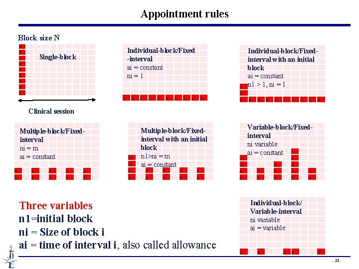
Appointment rules Block size N X X X X X Single-block X X X X X Individual-block/Fixed -interval ai = constant ni = 1 X X Individual-block/Fixed interval with an initial block ai = constant n 1 > 1, ni = 1 X X X X X Clinical session X X X X Multiple-block/Fixedinterval ni = m ai = constant X X X Multiple-block/Fixed- interval with an initial block n 1>ni = m ai = constant Three variables n 1=initial block ni = Size of block i ai = time of interval i, also called allowance Variable-block/Fixed interval ni variable ai = constant X X X X X Individual-block/ Variable-interval ni variable ai = variable X X X - 23 -

Appointment rules • Single-block rule : the most primitive “date only” AS ensuring doctor productivity by excessive patient waiting time. • Individual-block/Fixed-interval rule with an initial block : • Keep an inventory of patients to hedge against the risk of the unpunctuality or no-show of the 1 st patient • Bailey’s rule (n 1 = 2, ni = 1, ai = mean service time m-1) -> reasonable balance between patient waiting and doctor idle (1952) • Multiple-block/Fixed-interval rule : • Usually (ni = m, ai = mm-1) • Possibly more suitable when the mean consultation time is short (Nuffield Trust (1965)) • Lack of rigorous research on the circumstances multiple block rule performs better - 24 -

Appointment rules • Individual-block/Variable-interval rule: • The “dome” shape appointment intervals: initially increase toward the middle of the session and then decrease • Shown to be optimal for i. i. d. service times and uniform waiting costs for all patients - 25 -

Patient classification • Common model : homogenuous and served in FCFA (first-call first appointment) basis • Purposes of patient classification: sequence patients at booking, and adjust appointment intervals • Radiology examination times depend on factors such as patient’s age, physical mobility, and type of service. • Classification scheme: new/return, variability of service times (low/high-variance patients), and type of procedure • Limited interest in outpatient settings in which the schedule has to be ready in advance and the arriving requests are handled dynamically • Realistic application: the patients classified into a manageable number of groups and assigned to pre-marked slots when they call for appointments. Ex: new patients before 10: 00, return patients 10: 00 to 12: 00. • Drawback: reduced flexibility and potential lost capacity - 26 -

Adjustments • Whenever relevant, no-shows, walk-ins, urgent patients, and/or emergencies need to be planned for • No-shows cannot be entirely eliminated by administrative mechanisms • There is a tendency of walk-in aming lower social classes and it is not fair to deny walk-in access to clinics. • When the 2 nd consultation is frequent (orthopedics), some allowance should be made for the additional demand imposed on doctors • Suggestion from literature: the patient load (i. e. , percent of available appointments filled) be adjusted based on the expected number of walk-ins and no-shows. - 27 -

Adjustments • • Adjustment for no-shows None Overbooking extra patients to predetermined slots Decreasing appointment intervals proportionally • Adjustment for walk-ins, second consultations, urgent patients, and/or emergencies • None • Leaving some predetermined slots open • Increasing appointment intervals proportionally - 28 -

Adjustments • • Adjustment for no-shows None Overbooking extra patients to predetermined slots Decreasing appointment intervals proportionally • Adjustment for walk-ins, second consultations, urgent patients, and/or emergencies • None • Leaving some predetermined slots open • Increasing appointment intervals proportionally - 29 -

Analysis methodologies • Analystical studies • Queueing theory • Mathematical programming • Dynamic programming • Nonlinear programming • Stochastic programming • Simulation studies • Ho et al. (1992, 1999, 1995) evaluate 50 appointment rules under various operating environments. • No rule that performs well under all circumstances and a simple heuristic is proposed to choose an appointment rule for a clinic given p, CV, N, and Cp/Cd ratio • They find that p, CV, and N affect AS performance in the order of decreasing importance. - 30 -

Plan • Basis of Appointment Systems • Individual-block/Variable-interval rule • Variable-block/Fixed-interval rule • A static appointment model with dynamic features • Managing the Appointments with Waiting Time Targets and Random Walk-ins - 31 -

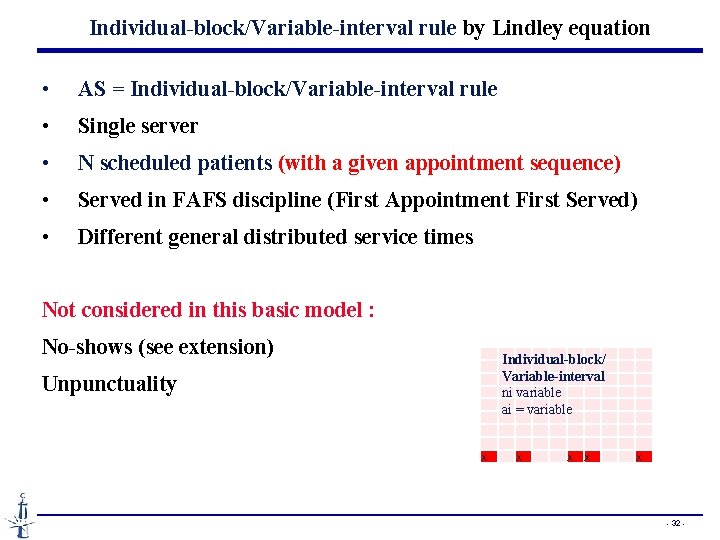
Individual-block/Variable-interval rule by Lindley equation • AS = Individual-block/Variable-interval rule • Single server • N scheduled patients (with a given appointment sequence) • Served in FAFS discipline (First Appointment First Served) • Different general distributed service times Not considered in this basic model : No-shows (see extension) Unpunctuality X Individual-block/ Variable-interval ni variable ai = variable X X X X - 32 -

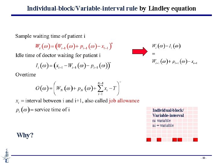
Individual-block/Variable-interval rule by Lindley equation Why? X Individual-block/ Variable-interval ni variable ai = variable X X X X - 33 -

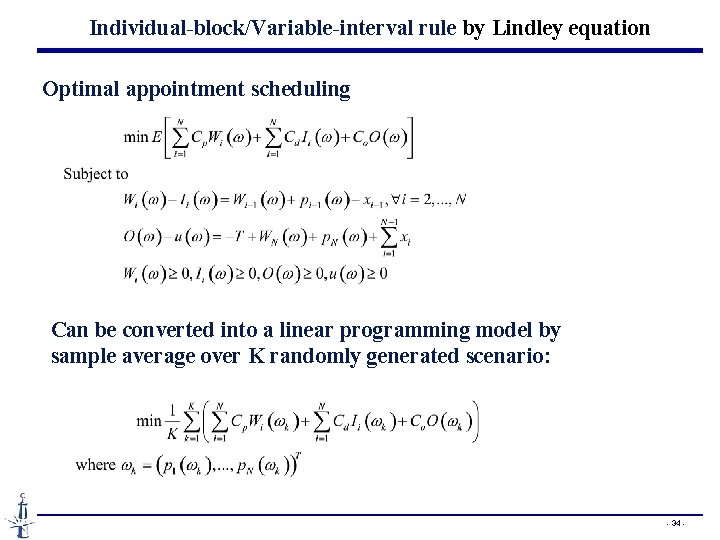
Individual-block/Variable-interval rule by Lindley equation Optimal appointment scheduling Can be converted into a linear programming model by sample average over K randomly generated scenario: - 34 -

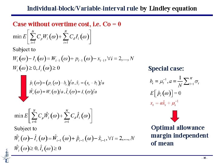
Individual-block/Variable-interval rule by Lindley equation Case without overtime cost, i. e. Co = 0 Special case: Optimal allowance margin independent of mean - 35 -

Individual-block/Variable-interval rule by Lindley equation Solution methods : • L-shape algorithm with sequence bounding in Denton & Gupta 2003 • Bender’s decomposition in Chen & Robinson 2014 • Stochastic approximation with sample path gradient (to be addressed in surgery scheduling part for a multi-server setting) - 36 -

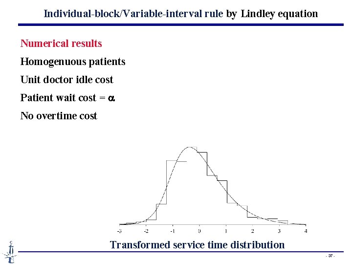
Individual-block/Variable-interval rule by Lindley equation Numerical results Homogenuous patients Unit doctor idle cost Patient wait cost = a No overtime cost Transformed service time distribution - 37 -

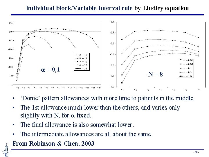
Individual-block/Variable-interval rule by Lindley equation a = 0, 1 N = 8 • ‘Dome’ pattern allowances with more time to patients in the middle. • The 1 st allowance much lower than the others, and varies only slightly with N, for a fixed. • The final allowance is also somewhat lower. • The intermediate allowances are all about the same. From Robinson & Chen, 2003 - 38 -

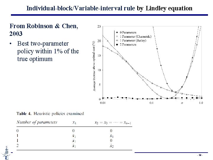
Individual-block/Variable-interval rule by Lindley equation From Robinson & Chen, 2003 • Best two-parameter policy within 1% of the true optimum - 39 -

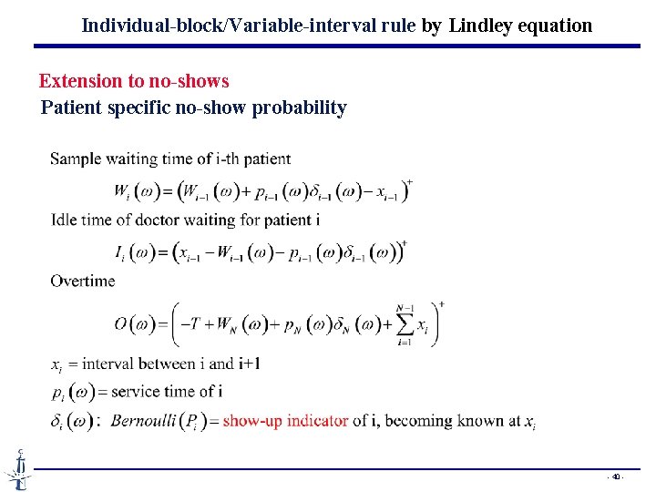
Individual-block/Variable-interval rule by Lindley equation Extension to no-shows Patient specific no-show probability - 40 -

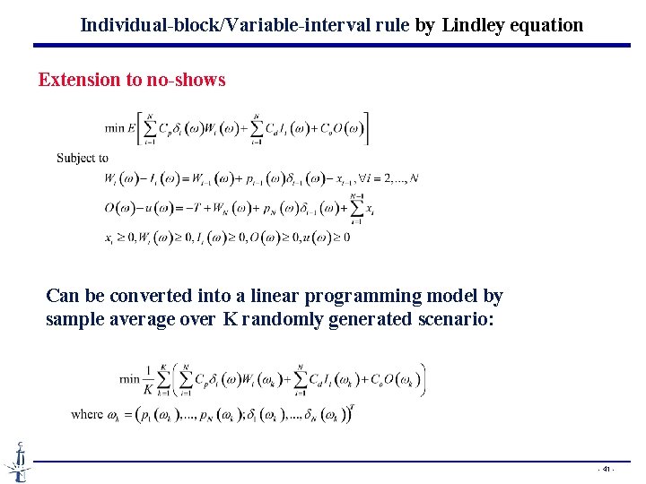
Individual-block/Variable-interval rule by Lindley equation Extension to no-shows Can be converted into a linear programming model by sample average over K randomly generated scenario: - 41 -

Plan • Basis of Appointment Systems • Individual-block/Variable-interval rule • Variable-block/Fixed-interval rule by queueing analysis • A static appointment model with dynamic features • Managing the Appointments with Waiting Time Targets and Random Walk-ins - 42 -

Variable-block/Fixed-interval rule by queueing analysis • AS = Variable-block/Fixed (or Given)-interval rule • Single server • N scheduled patients • Served in FAFS discipline (First Appointment First Served) • homogenuous patient population • Exponential service time distribution Not considered in this basic model : No-shows (see extension) Unpunctuality Walk-ins - 43 -

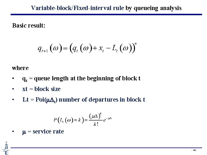
Variable-block/Fixed-interval rule by queueing analysis Basic result: where • qt = queue length at the beginning of block t • xt = block size • Lt = Poi(m. Dt) number of departures in block t • m = service rate - 44 -

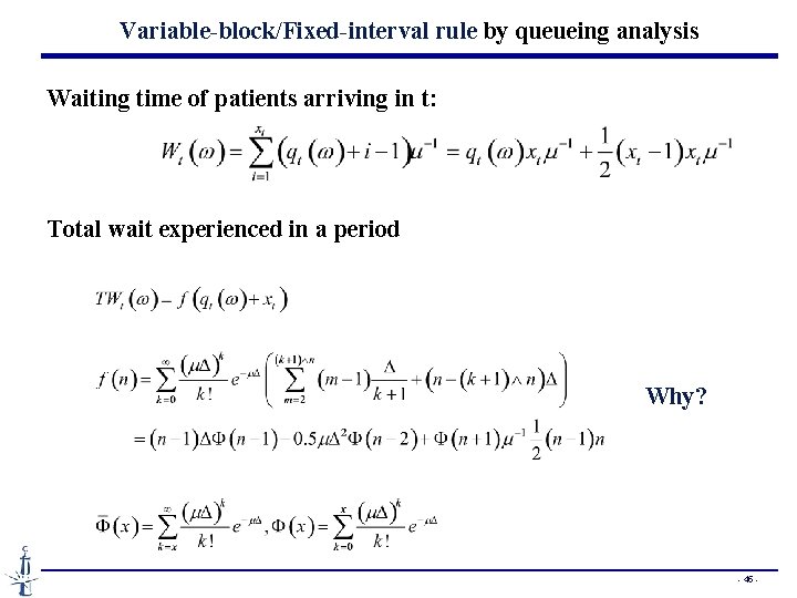
Variable-block/Fixed-interval rule by queueing analysis Waiting time of patients arriving in t: Total wait experienced in a period Why? - 45 -

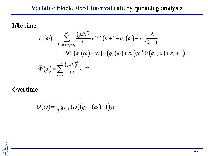
Variable-block/Fixed-interval rule by queueing analysis Idle time Overtime - 46 -

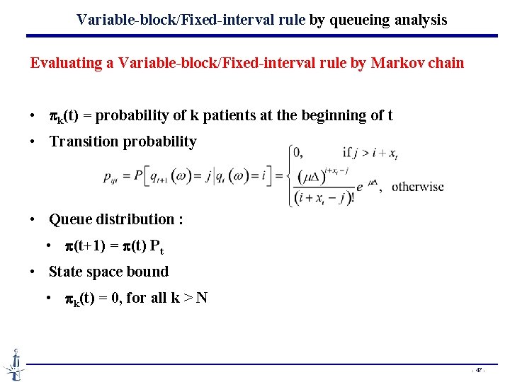
Variable-block/Fixed-interval rule by queueing analysis Evaluating a Variable-block/Fixed-interval rule by Markov chain • pk(t) = probability of k patients at the beginning of t • Transition probability • Queue distribution : • p(t+1) = p(t) Pt • State space bound • pk(t) = 0, for all k > N - 47 -

Variable-block/Fixed-interval rule by queueing analysis Optimal Variable-block/Fixed-interval rule • In some well-chosen neighborhood (Kaandorp & Koole, 2007), the cost function is multimodular in block size vector x and hence any local optimum is global optimum. - 48 -

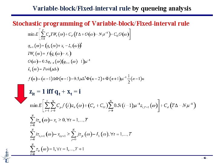
Variable-block/Fixed-interval rule by queueing analysis Stochastic programming of Variable-block/Fixed-interval rule zit = 1 iff qt + xt = i - 49 -

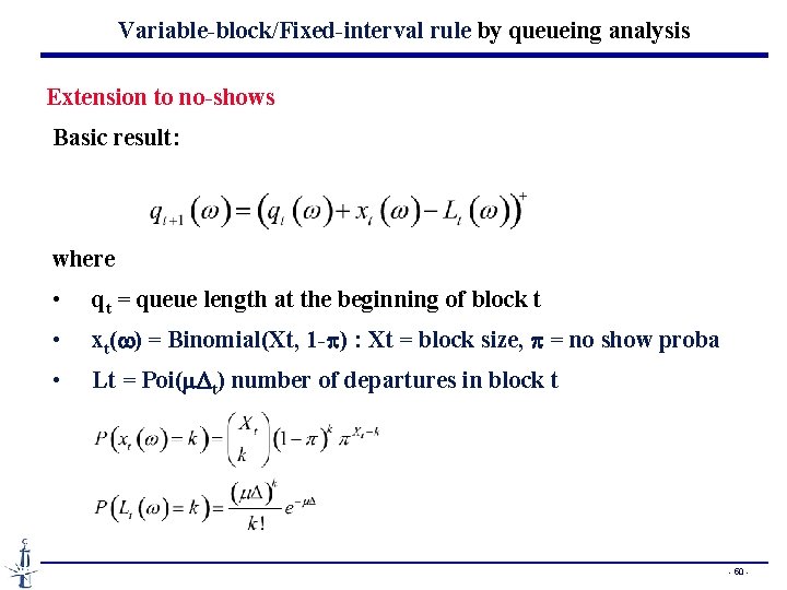
Variable-block/Fixed-interval rule by queueing analysis Extension to no-shows Basic result: where • qt = queue length at the beginning of block t • xt(w) = Binomial(Xt, 1 -p) : Xt = block size, p = no show proba • Lt = Poi(m. Dt) number of departures in block t - 50 -

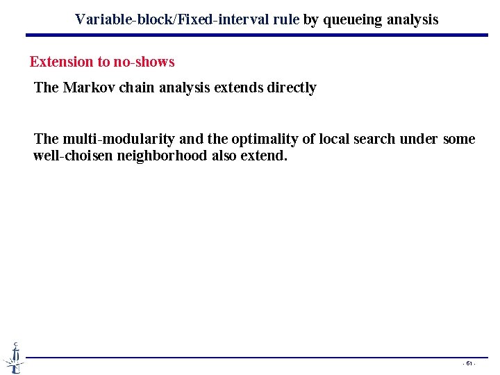
Variable-block/Fixed-interval rule by queueing analysis Extension to no-shows The Markov chain analysis extends directly The multi-modularity and the optimality of local search under some well-choisen neighborhood also extend. - 51 -

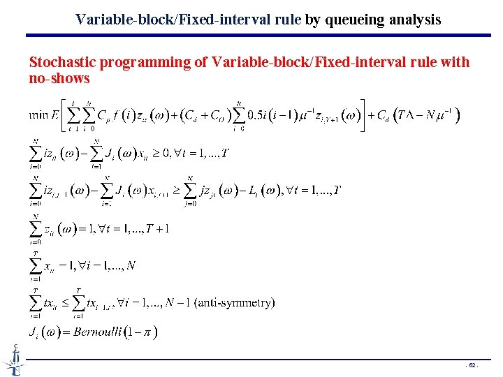
Variable-block/Fixed-interval rule by queueing analysis Stochastic programming of Variable-block/Fixed-interval rule with no-shows - 52 -

Plan • Basis of Appointment Systems • Individual-block/Variable-interval rule • Variable-block/Fixed-interval rule • A static appointment model with dynamic features • Managing the Appointments with Waiting Time Targets and Random Walk-ins - 53 -

From Kumar Muthuraman, Mark Lawley, « A stochastic overbooking model for outpatient clinical scheduling with no-shows » IIE Transactions, 40, 820 -837, 2008 A static appointment model with many dynamic features - 54 -

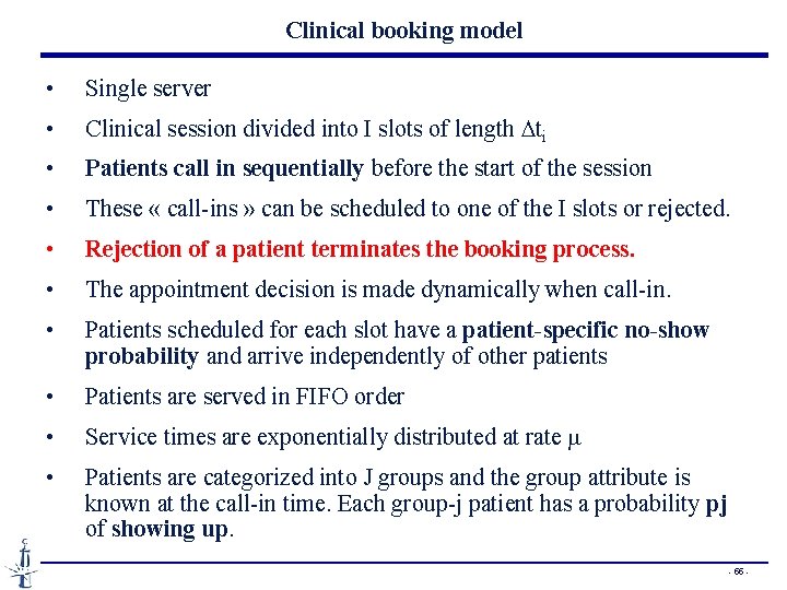
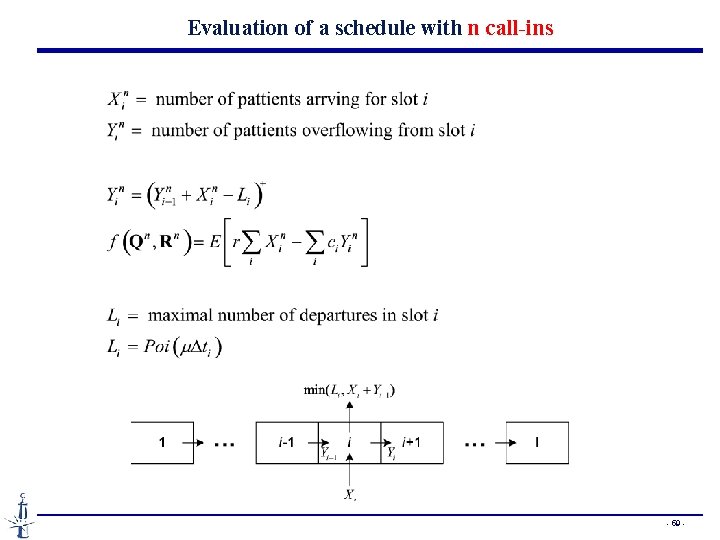
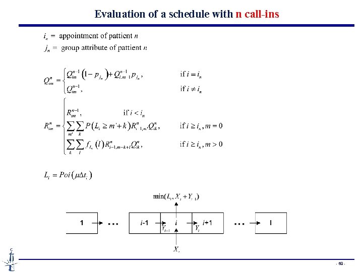
Clinical booking model • Single server • Clinical session divided into I slots of length Dti • Patients call in sequentially before the start of the session • These « call-ins » can be scheduled to one of the I slots or rejected. • Rejection of a patient terminates the booking process. • The appointment decision is made dynamically when call-in. • Patients scheduled for each slot have a patient-specific no-show probability and arrive independently of other patients • Patients are served in FIFO order • Service times are exponentially distributed at rate m • Patients are categorized into J groups and the group attribute is known at the call-in time. Each group-j patient has a probability pj of showing up. - 55 -

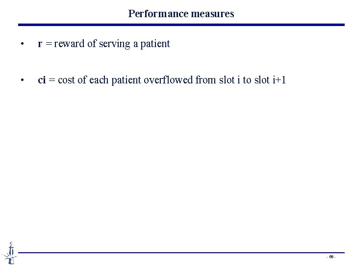
Performance measures • r = reward of serving a patient • ci = cost of each patient overflowed from slot i to slot i+1 - 56 -

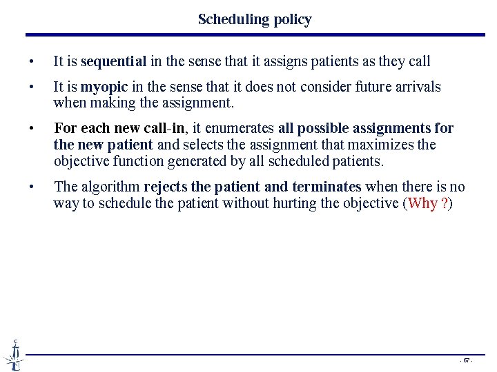
Scheduling policy • It is sequential in the sense that it assigns patients as they call • It is myopic in the sense that it does not consider future arrivals when making the assignment. • For each new call-in, it enumerates all possible assignments for the new patient and selects the assignment that maximizes the objective function generated by all scheduled patients. • The algorithm rejects the patient and terminates when there is no way to schedule the patient without hurting the objective (Why ? ) - 57 -

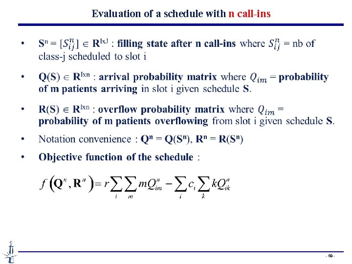
Evaluation of a schedule with n call-ins - 58 -

Evaluation of a schedule with n call-ins - 59 -

Evaluation of a schedule with n call-ins - 60 -

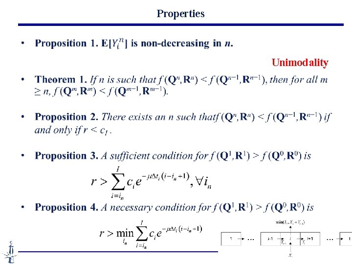
Properties Unimodality - 61 -

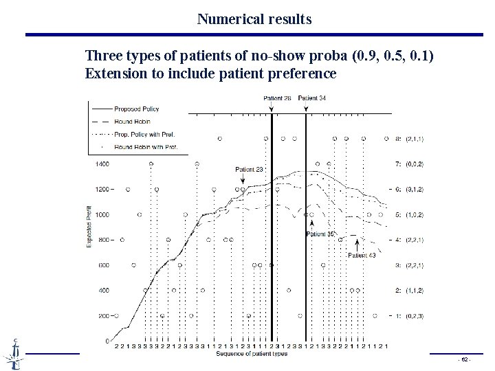
Numerical results Three types of patients of no-show proba (0. 9, 0. 5, 0. 1) Extension to include patient preference - 62 -

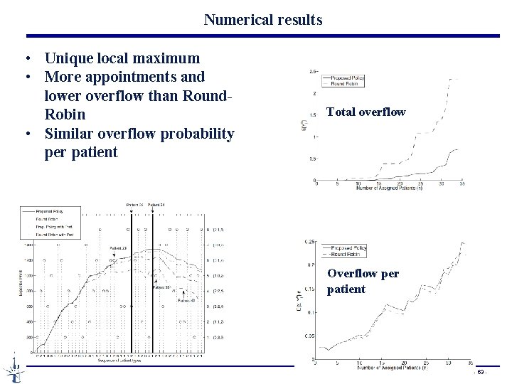
Numerical results • Unique local maximum • More appointments and lower overflow than Round. Robin • Similar overflow probability per patient Total overflow Overflow per patient - 63 -

Plan • Basis of Appointment Systems • Individual-block/Variable-interval rule • Variable-block/Fixed-interval rule • A static appointment model with dynamic features • Managing the Appointments with Waiting Time Targets and Random Walk-ins - 64 -

From Xingwei Pan, Na Geng, Xiaolan Xie, Jing Wen, « Managing appointments with waiting time targets and random walk-ins”, submitted - 65 -