Chapter 2 A basic overview of statistical tests

Chapter 2 A basic overview of statistical tests that are used commonly Vamsi Balakrishnan

Statistical Tests • Purpose • Major (common) Tests – Student’s t-Test (paired or independent) – Wilcoxon Mann-Whitney rank sum test – Wilcoxon signed rank test – Contingency tables (Chi-square tests) – Mc. Nemar’s Test • Assumptions

Normal Populations • Student’s t-Test • Two types – Independent – Paired

Independent Student’s t-Test [equal variance] • H 0: μ 1 = μ 2 • HA: <not above> • Assumptions – Normality – Equal Variance – Independent samples • Same standard deviation (and hence variance) is assumed for both sample populations. • “The test statistic is essentially a standardized difference of the two sample means. ”

Independent Student’s t-Test (continued) [equal variance] • The Test Statistic (t-statistic) • X and Y are the two populations. The bar above it means sample mean. • The n 1 and n 2 are the sample sizes. • Sp = pooled standard deviation.

Independent Student’s t-Test (continued) [equal variance] • Sp = Pooled Standard deviation – Purpose – Computational Formula: – n 1 and n 2 are the sample sizes, si are the standard deviations for the population.

Independent Student’s t-Test (continued) [equal variance] • Degrees of Freedom – The possibilities (opportunities) for change – 1 usually. Here though… – n 1+n 2 -2

Independent Student’s t-Test (unequal/difference variances) • Modified t statistic • Welch Test – Same assumptions as previous test (independence, normality) except, unequal variance – Same hypotheses are used – Compare to previous equal var. formula • Used for data of very different sizes (Relative definition)

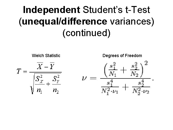
Independent Student’s t-Test (unequal/difference variances) (continued) Welch Statistic Degrees of Freedom

Paired Student’s t-Test • “paired t-test I used to compare the means of two populations” when the data is paired: – Before-and-after – Same individual is observed twice • Null Hypothesis – H 0 = 0 – Ha = <not above>

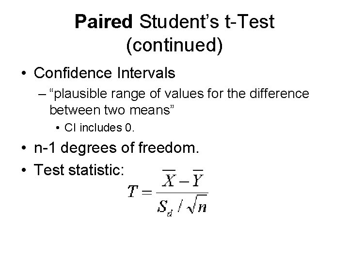
Paired Student’s t-Test (continued) • Confidence Intervals – “plausible range of values for the difference between two means” • CI includes 0. • n-1 degrees of freedom. • Test statistic:

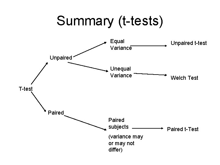
Summary (t-tests) Equal Variance Unpaired t-test Unpaired Unequal Variance Welch Test T-test Paired subjects (variance may or may not differ) Paired t-Test

Non-Parametric • No distribution • Paired vs. Unpaired • Types: – Wilcoxon Mann-Whitney Rank Sum Test – Wilcoxon signed rank test

Wilcoxon Mann-Whitney Rank Sum Test • T-statistic applied to the ranks, not data • Intended for not-normal (non-parametric), but independent • Hypothesis – H 0 – “the two populations being compared have identical distributions” – HA – “populations differ in location i. e. (median)”

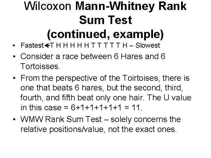
Wilcoxon Mann-Whitney Rank Sum Test (continued, example) • Fastest - T H H H T T T H – Slowest • Consider a race between 6 Hares and 6 Tortoisses. • From the perspective of the Toirtoises, there is one that beats 6 hares, but the second, third, fourth, and fifth beat only one hair. The U value in this case = 6+1+1+1 = 11. • WMW Rank Sum Test – solely concerns the relative positions/value, not the exact ones.

Paired Wilcoxin Test • Two-sample version of the previous test except that the individuals may be measured twice or before-and-after measurements may be considered.

Paired Wilcoxin Test (continued) • Computing the U-statistic is very easy. • This test should only be done on data that has the same number of measurements. • Create a third column – If the difference between the “before” – “after” is positive, then put a + sign. – If the difference is “negative” put a negative sign. – Add up all of these signs, the resulting positive or negative value is the statistic. • Consider ns/r = Xa. Xb possible – number of pairs of Xa-Xb=0 pairs. – ns/r > 10: sampling dist is close to normal

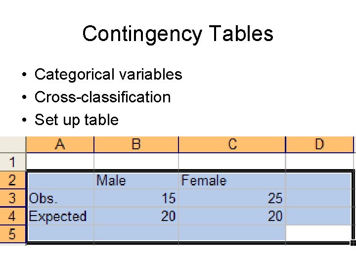
Contingency Tables • Categorical variables • Cross-classification • Set up table

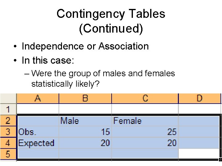
Contingency Tables (Continued) • Independence or Association • In this case: – Were the group of males and females statistically likely?

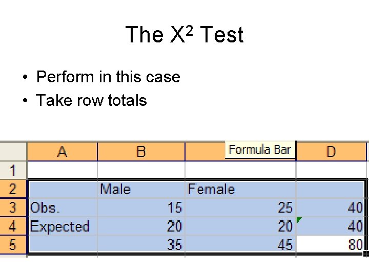
The X 2 Test • Perform in this case • Take row totals

The X 2 Test (Continued) • [(15 -20)^2/20] + [(25 -20)^2/20)] = 2. 5 = X 2 • Degrees of freedom = n-1 = 2 -1 = 1

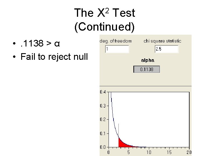
The X 2 Test (Continued) • . 1138 > α • Fail to reject null

Mc. Nemar’s Test • Categorical data from paired observations • “…cases matched with controls on variables such as sex, age, and so on, or observations made on the same subjects on two occasions (cf. paired t-test). ” • Hypothesis – H 0: populations do not differ

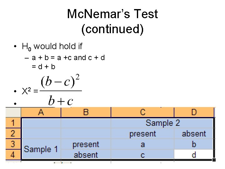
Mc. Nemar’s Test (continued) • H 0 would hold if – a + b = a +c and c + d =d+b • X 2 = •

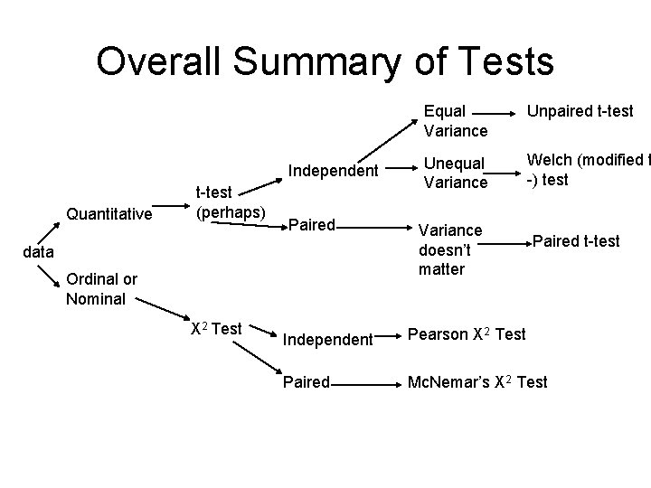
Overall Summary of Tests Independent Quantitative t-test (perhaps) Paired data Ordinal or Nominal X 2 Test Equal Variance Unpaired t-test Unequal Variance Welch (modified t -) test Variance doesn’t matter Paired t-test Independent Pearson X 2 Test Paired Mc. Nemar’s X 2 Test