Chapter 19 Population Ecology Power Point Lectures for

Chapter 19 Population Ecology Power. Point® Lectures for Campbell Essential Biology, Fourth Edition – Eric Simon, Jane Reece, and Jean Dickey Campbell Essential Biology with Physiology, Third Edition – Eric Simon, Jane Reece, and Jean Dickey Lectures by Chris C. Romero, updated by Edward J. Zalisko © 2010 Pearson Education, Inc.

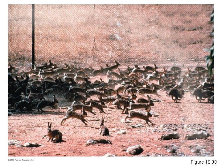
Biology and Society: Multiplying Like Rabbits • In 1859, 12 pairs of European rabbits were released on a ranch in southern Australia. • By 1865, 20, 000 rabbits were killed on just that one ranch. • By 1900, several hundred million rabbits were distributed over most of the continent. © 2010 Pearson Education, Inc.

Figure 19. 00

• The European rabbits – Destroyed farming and grazing land – Promoted soil erosion – Made grazing treacherous for cattle and sheep – Competed directly with native marsupials © 2010 Pearson Education, Inc.

• The European red fox – Was introduced to control the rabbits – Spread across Australia – Ate several species of native birds and small mammals to extinction – Had little impact on the rabbit population © 2010 Pearson Education, Inc.

• Today, rabbits, foxes, and a long list of other non-native animal and plant species are – Still entrenched in Australia – Damaging the environment – Costing hundreds of millions of dollars in economic losses © 2010 Pearson Education, Inc.

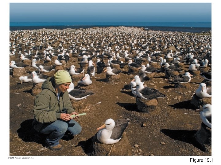
AN OVERVIEW OF POPULATION ECOLOGY • Population ecology is the study of factors that affect population: – Density – Growth • A population is a group of individuals of a single species that occupy the same general area. © 2010 Pearson Education, Inc.

• Population ecology focuses on the factors that influence a population’s – Density – Structure – Size – Growth rate © 2010 Pearson Education, Inc.

Figure 19. 1

• Population ecology is used to study – How to develop sustainable fisheries – How to control pests and pathogens – Human population growth © 2010 Pearson Education, Inc.

Population Density • Population density is the number of individuals of a species per unit of area or volume. Examples include – The number of largemouth bass per cubic kilometer (km 3) of a lake – The number of oak trees per square kilometer (km 2) in a forest – The number of nematodes per cubic meter (m 3) in a forest’s soil © 2010 Pearson Education, Inc.

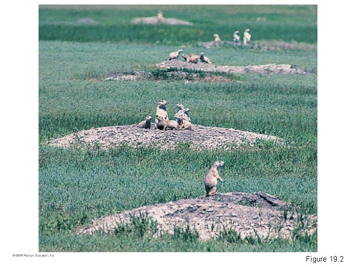
• How do we measure population density? – In most cases, it is impractical or impossible to count all individuals in a population. – In some cases, population densities are estimated by indirect indicators, such as – Number of bird nests – Rodent burrows © 2010 Pearson Education, Inc.

Figure 19. 2

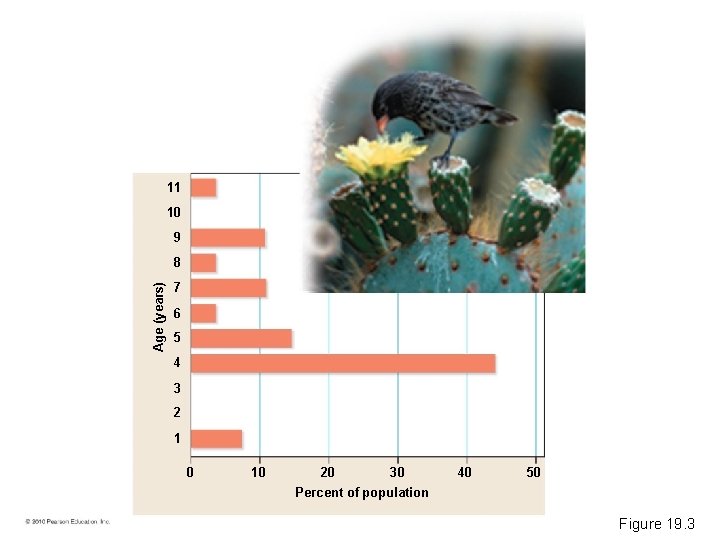
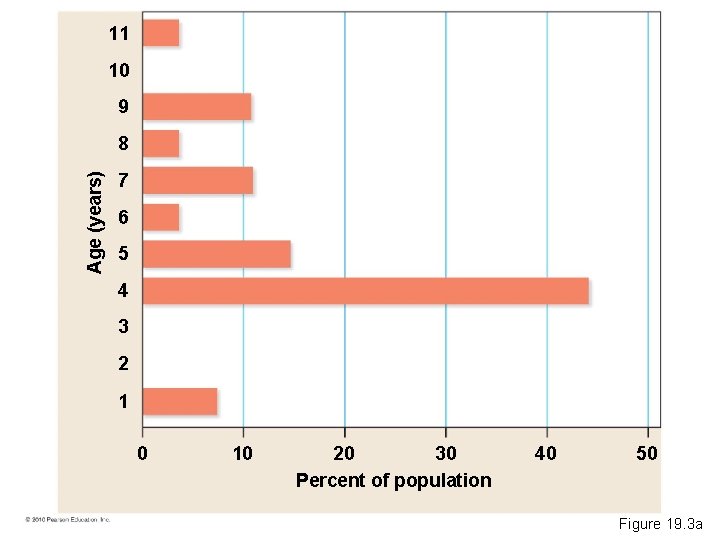
Population Age Structure • The age structure of a population is the distribution of individuals among age groups. • The age structure of a population provides insight into – The history of a population’s survival – Reproductive success – How the population relates to environmental factors © 2010 Pearson Education, Inc.

11 10 9 Age (years) 8 7 6 5 4 3 2 1 0 10 20 30 40 50 Percent of population Figure 19. 3

11 10 9 Age (years) 8 7 6 5 4 3 2 1 0 10 20 30 Percent of population 40 50 Figure 19. 3 a

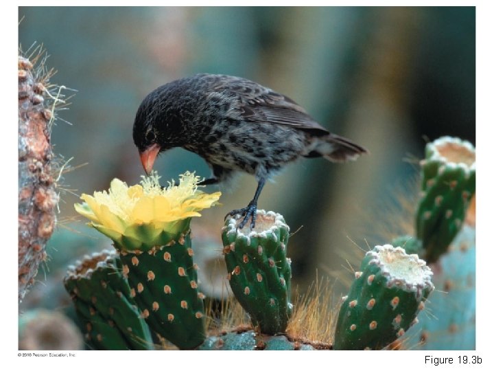
Figure 19. 3 b

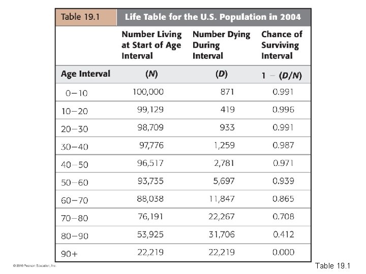
Life Tables and Survivorship Curves • Life tables – Track survivorship – Help to determine the most vulnerable stages of the life cycle © 2010 Pearson Education, Inc.

Table 19. 1

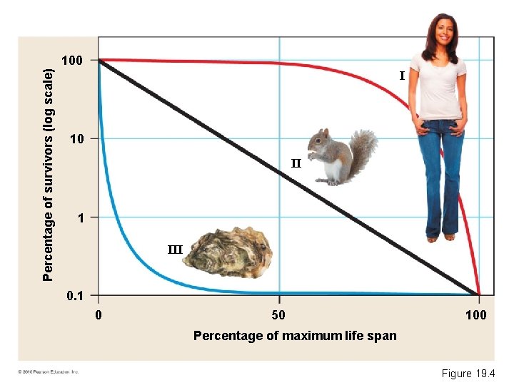
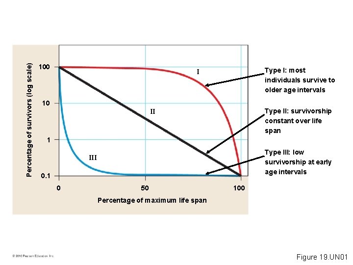
• Survivorship curves – Graphically represent some of the data in a life table – Are classified based upon the rate of mortality over the life span of an organism © 2010 Pearson Education, Inc.

Percentage of survivors (log scale) 100 I 10 II 1 III 0. 1 0 50 100 Percentage of maximum life span Figure 19. 4

Life History Traits as Evolutionary Adaptations • An organism’s life history is the set of traits that affect the organism’s schedule of – Reproduction – Survival © 2010 Pearson Education, Inc.

• Key life history traits are the – Age at first reproduction – Frequency of reproduction – Number of offspring – Amount of parental care provided © 2010 Pearson Education, Inc.

• Life history traits – Evolve – Represent a compromise of the competing needs for – Time – Energy – Nutrients © 2010 Pearson Education, Inc.

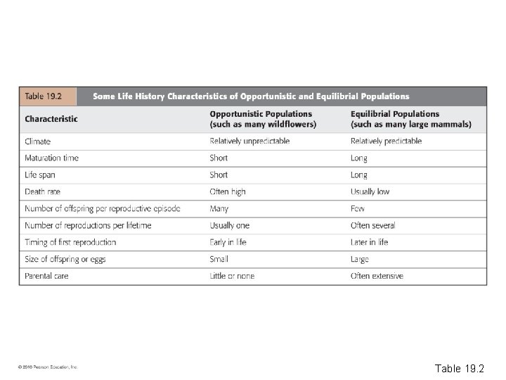
• Organisms with an opportunistic life history – Take immediate advantage of favorable conditions – Typically exhibit a Type III survivorship curve © 2010 Pearson Education, Inc.

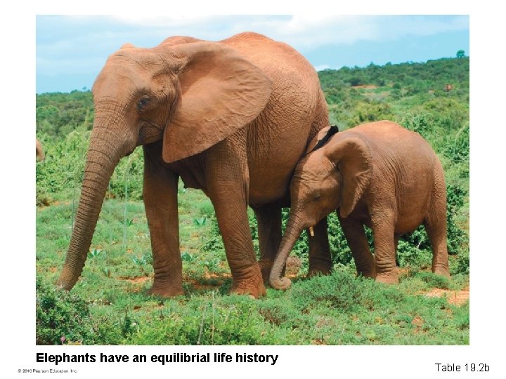
• Organisms with an equilibrial life history – Reach sexual maturity slowly – Produce few, well cared for offspring – Are typically large-bodied and longer lived – Typically exhibit a Type I survivorship curve © 2010 Pearson Education, Inc.

Table 19. 2

Dandelions have an opportunistic life history Table 19. 2 a

Elephants have an equilibrial life history Table 19. 2 b

POPULATION GROWTH MODELS • Population size fluctuates as individuals – Are born – Immigrate into an area – Emigrate away – Die © 2010 Pearson Education, Inc.

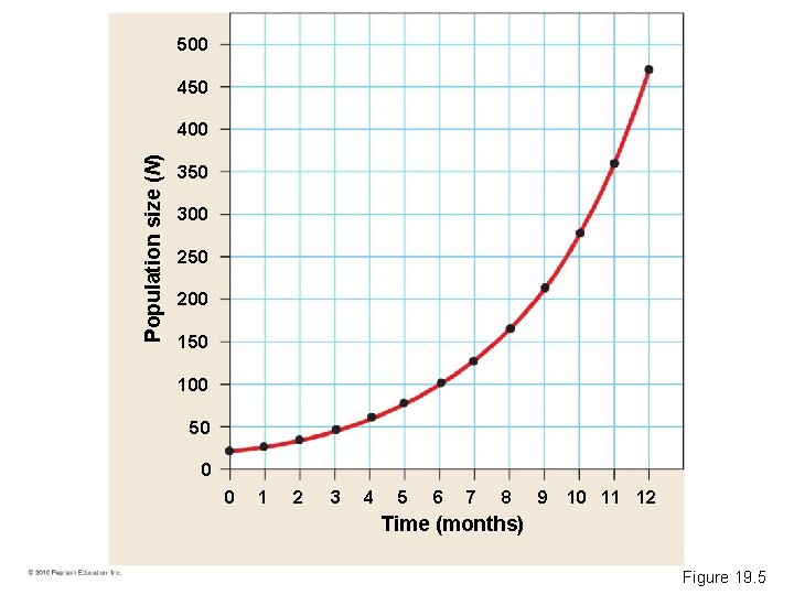
The Exponential Growth Model: The Ideal of an Unlimited Environment • Exponential population growth describes the expansion of a population in an ideal and unlimited environment. © 2010 Pearson Education, Inc.

500 450 Population size (N) 400 350 300 250 200 150 100 50 0 0 1 2 3 4 5 6 7 8 9 10 11 12 Time (months) Figure 19. 5

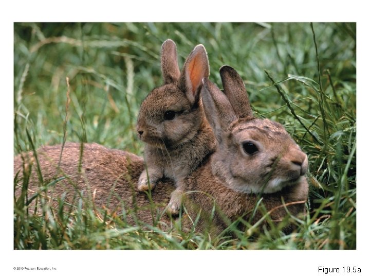
Figure 19. 5 a

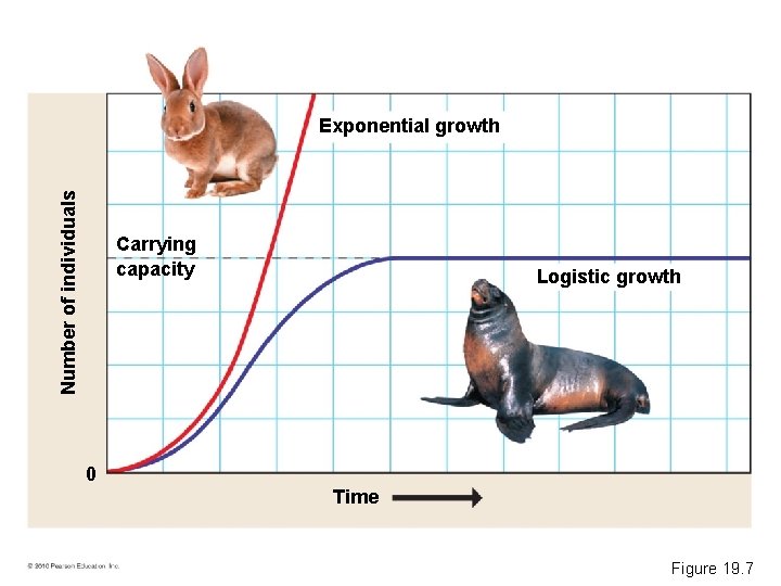
• Exponential growth explains how – A few dozen rabbits can multiple into millions – In certain circumstances following disasters, organisms that have opportunistic life history patterns can rapidly recolonize a habitat © 2010 Pearson Education, Inc.

The Logistic Growth Model: The Reality of a Limited Environment • Limiting factors – Are environmental factors that hold population growth in check – Restrict the number of individuals that can occupy a habitat © 2010 Pearson Education, Inc.

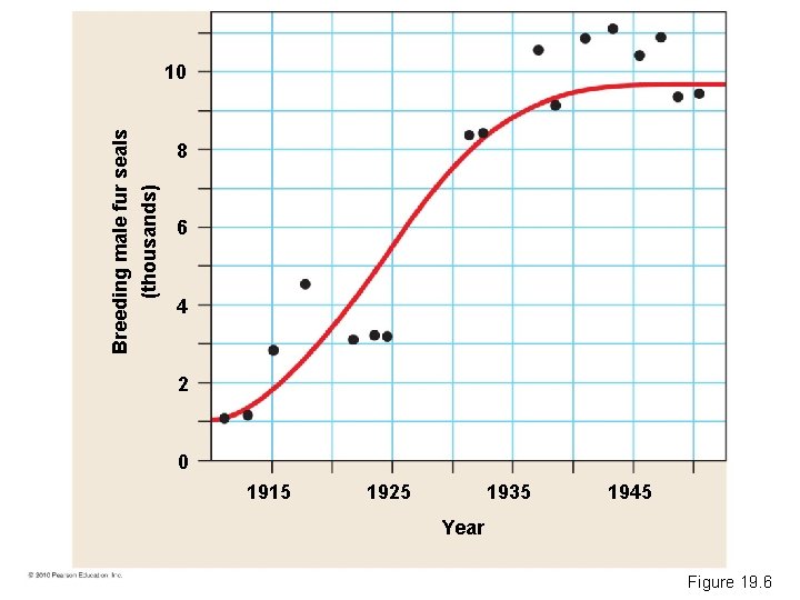
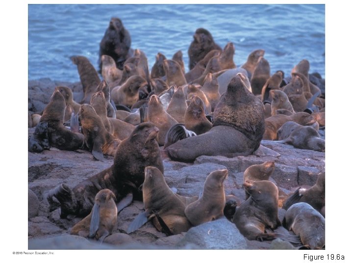
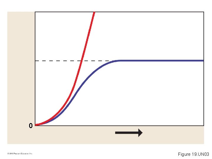
• The carrying capacity is the maximum population size that a particular environment can sustain. • Logistic population growth occurs when the growth rate decreases as the population size approaches carrying capacity. © 2010 Pearson Education, Inc.

Breeding male fur seals (thousands) 10 8 6 4 2 0 1915 1925 1935 1945 Year Figure 19. 6

Figure 19. 6 a

• The carrying capacity for a population varies, depending on – The species – The resources available in the habitat © 2010 Pearson Education, Inc.

• Organisms exhibiting equilibrial life history patterns occur in environments where the population size is at or near carrying capacity. © 2010 Pearson Education, Inc.

• The logistic model and the exponential model are theoretical ideals of population growth. • No natural population fits either one perfectly. © 2010 Pearson Education, Inc.

Number of individuals Exponential growth Carrying capacity Logistic growth 0 Time Figure 19. 7

Regulation of Population Growth Density-Dependent Factors • The logistic model is a description of intraspecific competition, competition between individuals of the same species for the same limited resources. © 2010 Pearson Education, Inc.

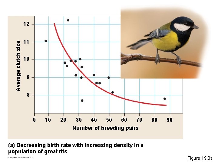
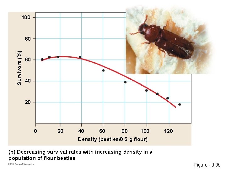
• As population size increases – Competition becomes more intense – The growth rate declines in proportion to the intensity of competition • A density-dependent factor is a population-limiting factor whose effects intensify as the population increases in density. Video: Chimp Agonistic Behavior Video: Snake Ritual Wrestling Video: Wolves Agonistic Behavior © 2010 Pearson Education, Inc.

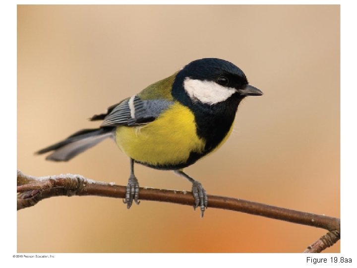
Average clutch size 12 11 10 9 8 0 10 20 30 40 50 60 70 80 90 Number of breeding pairs (a) Decreasing birth rate with increasing density in a population of great tits Figure 19. 8 a

Figure 19. 8 aa

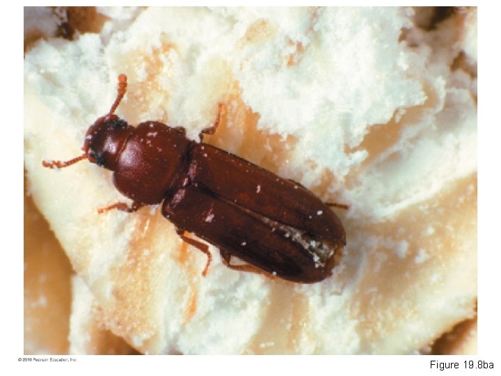
100 Survivors (%) 80 60 40 20 40 60 80 100 120 Density (beetles/0. 5 g flour) (b) Decreasing survival rates with increasing density in a population of flour beetles Figure 19. 8 b

Figure 19. 8 ba

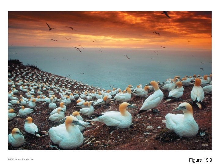
• Density-dependent factors may include – Accumulation of toxic wastes – Limited food supply – Limited territory © 2010 Pearson Education, Inc.

Figure 19. 9

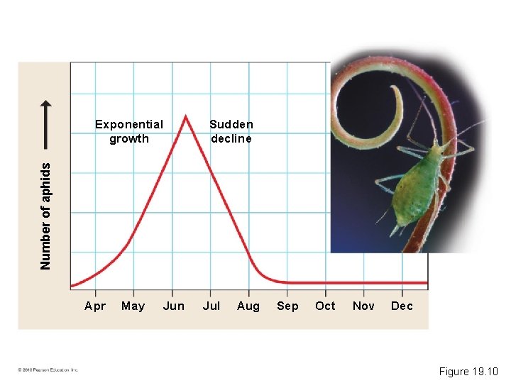
Density-Independent Factors • Density-independent factors – Are population-limiting factors whose intensity is unrelated to population density – Include abiotic factors such as – Fires – Floods – Storms Video: Albatross Courtship Ritual Video: Blue-footed Boobies Courtship Ritual Video: Giraffe Courtship Ritual © 2010 Pearson Education, Inc.

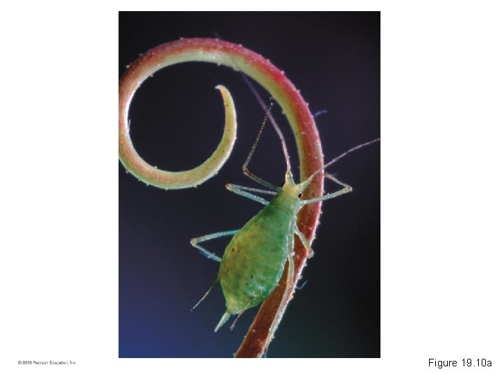
Sudden decline Number of aphids Exponential growth Apr May Jun Jul Aug Sep Oct Nov Dec Figure 19. 10

Figure 19. 10 a

• In many natural populations, density-independent factors limit population size before density-dependent factors become important. • Over the long term, most populations are probably regulated by a mixture of – Density-independent factors – Density-dependent factors © 2010 Pearson Education, Inc.

Population Cycles • Some populations have regular boom-and-bust cycles characterized by periods of rapid growth followed by steep population declines. © 2010 Pearson Education, Inc.

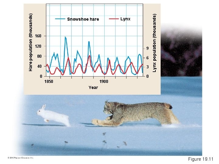
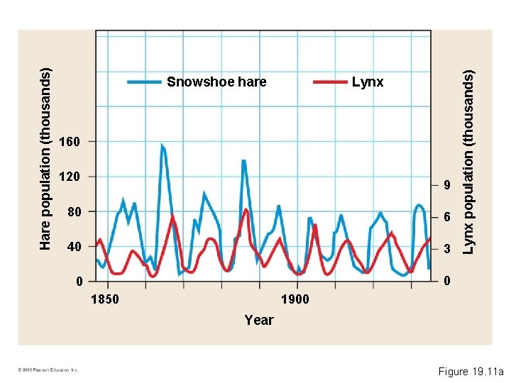
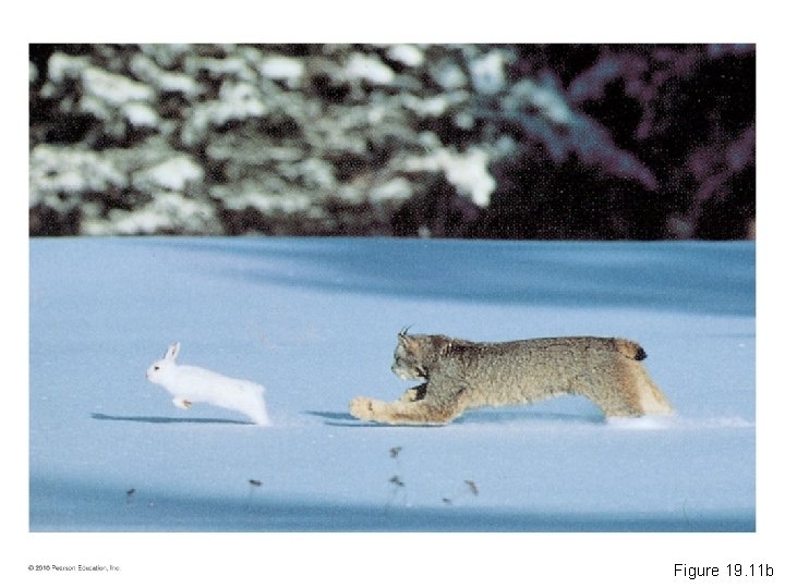
• A well studied example of boom and bust cycles are the cycles of – Snowshoe hares – One of the hares’ predators, the lynx © 2010 Pearson Education, Inc.

160 120 9 80 6 40 3 0 0 1850 Lynx population (thousands) Hare population (thousands) Lynx Snowshoe hare 1900 Year Figure 19. 11

Lynx 160 120 9 80 6 40 3 0 0 1850 Lynx population (thousands) Hare population (thousands) Snowshoe hare 1900 Year Figure 19. 11 a

Figure 19. 11 b

• The cause of these hare and lynx cycles may be – Winter food shortages for the hares – Overexploitation of hares by lynx – A combination of both of these mechanisms © 2010 Pearson Education, Inc.

APPLICATIONS OF POPULATION ECOLOGY • Population ecology is used to – Increase populations of organisms we wish to harvest – Decrease populations of pests – Save populations of organisms threatened with extinction © 2010 Pearson Education, Inc.

Conservation of Endangered Species • The U. S. Endangered Species Act defines – An endangered species as one that is in danger of extinction throughout all or a significant portion of its range – A threatened species as one that is likely to become endangered in the foreseeable future © 2010 Pearson Education, Inc.

• A major factor in population decline is habitat destruction or modification. © 2010 Pearson Education, Inc.

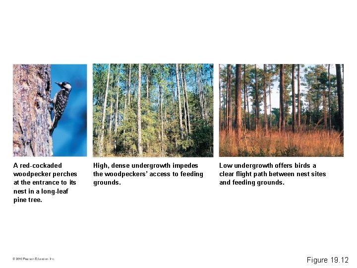
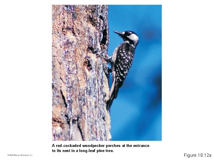
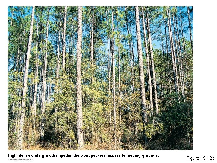
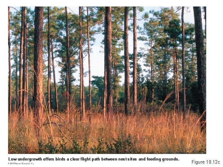
• The red-cockaded woodpecker – Requires longleaf pine forests with clear flight paths between trees – Suffered from fire suppression, increasing the height of the vegetation on the forest floor – Recovered from near-extinction to sustainable populations due to controlled burning and other management methods © 2010 Pearson Education, Inc.

A red-cockaded woodpecker perches at the entrance to its nest in a long-leaf pine tree. High, dense undergrowth impedes the woodpeckers’ access to feeding grounds. Low undergrowth offers birds a clear flight path between nest sites and feeding grounds. Figure 19. 12

A red-cockaded woodpecker perches at the entrance to its nest in a long-leaf pine tree. Figure 19. 12 a

High, dense undergrowth impedes the woodpeckers’ access to feeding grounds. Figure 19. 12 b

Low undergrowth offers birds a clear flight path between nest sites and feeding grounds. Figure 19. 12 c

Sustainable Resource Management • According to the logistic growth model, the fastest growth rate occurs when a population size is at roughly half the carrying capacity. © 2010 Pearson Education, Inc.

• Theoretically, populations should be harvested down to this level, assuming that growth rate and carrying capacity are stable over time. © 2010 Pearson Education, Inc.

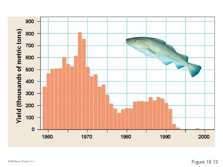
• In the northern Atlantic cod fishery – Estimates of cod stocks were too high – The practice of discarding young cod (not of legal size) at sea caused a higher mortality rate than was predicted – The fishery collapsed in 1992 and has not recovered © 2010 Pearson Education, Inc.

Yield (thousands of metric tons) 900 800 700 600 500 400 300 200 100 0 1960 1970 1980 1990 2000 Figure 19. 13

Invasive Species • An invasive species – Is a non-native species that has spread far beyond the original point of introduction – Causes environmental or economic damage by colonizing and dominating suitable habitats • In the United States, invasive species cost about $137 billion a year. © 2010 Pearson Education, Inc.

• Invasive species typically exhibit an opportunistic life history pattern. © 2010 Pearson Education, Inc.

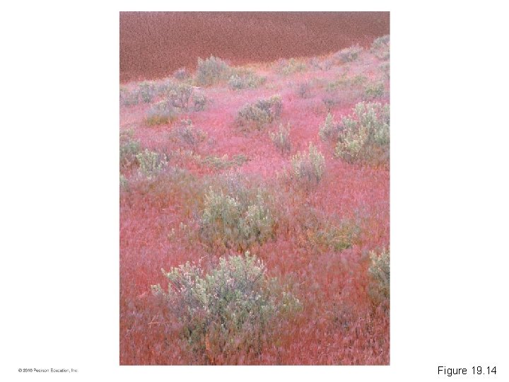
• Cheatgrass – Is an invasive species in the western United States – Currently covers more than 60 million acres of rangeland formerly dominated by native grasses and sagebrush – Produces seeds earlier and in greater abundance than native species – Forms highly flammable brush creating fires that native plants cannot tolerate © 2010 Pearson Education, Inc.

Figure 19. 14

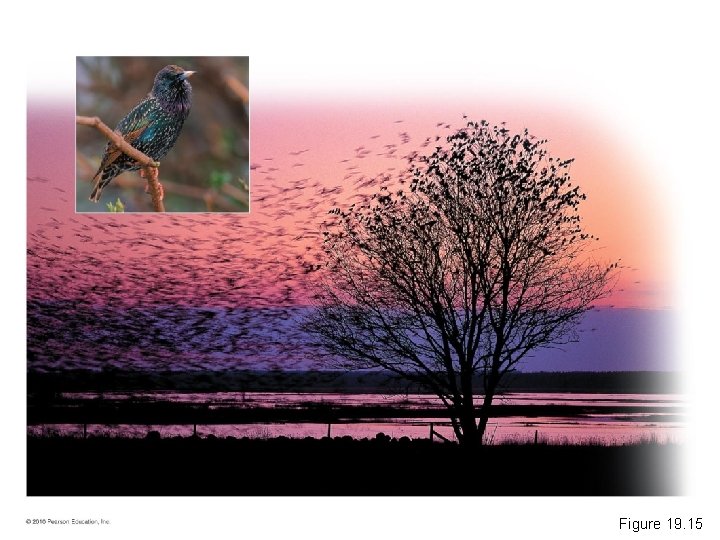
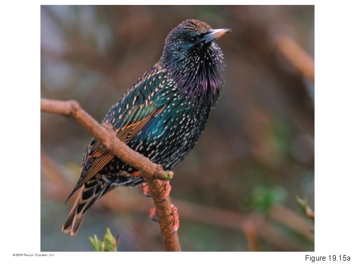
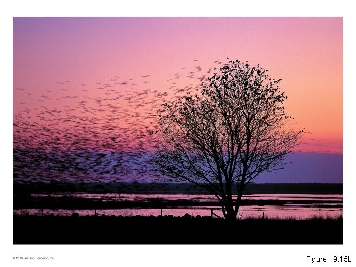
• European starlings – Are another invasive species – Were first released into New York in 1890 – Now number more than 200 million in the United States © 2010 Pearson Education, Inc.

Figure 19. 15

Figure 19. 15 a

Figure 19. 15 b

Biological Control of Pests • Invasive species may benefit from the absence of – Pathogens – Predators – Herbivores • Biological control – Is the intentional release of a natural enemy to attack a pest population – Is used to manage an invasive species © 2010 Pearson Education, Inc.

• In 1950, the Australian government introduced a virus lethal to European rabbits into the rabbits’ Australian environment. © 2010 Pearson Education, Inc.

• Although initially successful, natural selection favored – Resistant rabbits – Variations of the virus that – Were not fatal or – Killed their hosts more slowly © 2010 Pearson Education, Inc.

• Evolutionary changes such as these, in which an adaptation of one species leads to a counteradaptation in a second species, are known as coevolution. © 2010 Pearson Education, Inc.

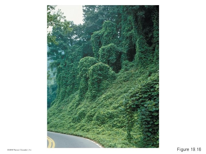
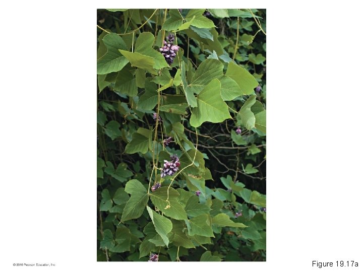
The Process of Science: Can Biological Control Defeat Kudzu? • Kudzu – Is an invasive Asian vine – Covers about 12, 000 square miles of the southeastern United States – Has a range limited by cold winters © 2010 Pearson Education, Inc.

Figure 19. 16

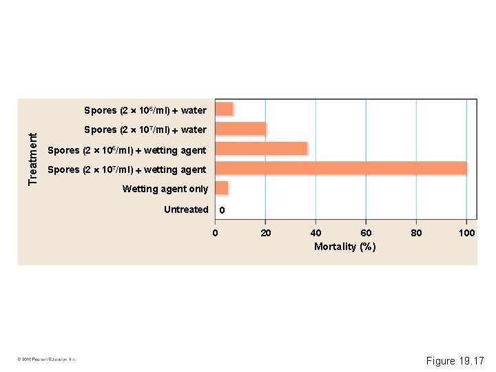
• Many strategies to control kudzu have been considered with little success. • A fungal pathogen called Myrothecium verrucaria appears to be a promising candidate for biological control. © 2010 Pearson Education, Inc.

• Observation: The fungus Myrothecium verrucaria causes severe disease in other weeds belonging to the same family as kudzu. • Question: Will the application of fungal spores of M. verrucaria control an established stand of kudzu in a natural setting? • Hypothesis: M. verrucaria treatment that was effective in small outdoor plantings would also be most effective in a natural setting. © 2010 Pearson Education, Inc.

• Prediction: The greatest kudzu mortality would result from the treatment that sprayed the highest concentration of spores in combination with a wetting agent. • Results: The hypothesis was supported by the data, as indicated in the following table. © 2010 Pearson Education, Inc.

Treatment Spores (2 106/ml) water Spores (2 107/ml) water Spores (2 106/ml) wetting agent Spores (2 107/ml) wetting agent Wetting agent only Untreated 0 0 20 40 60 80 100 Mortality (%) Figure 19. 17

Figure 19. 17 a

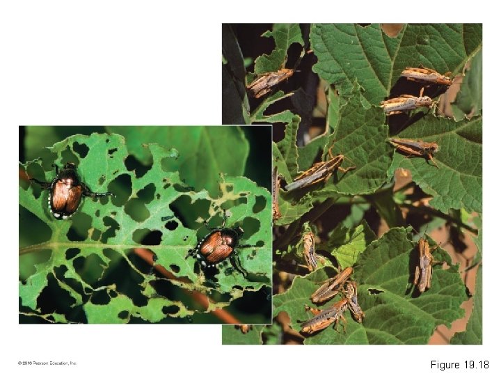
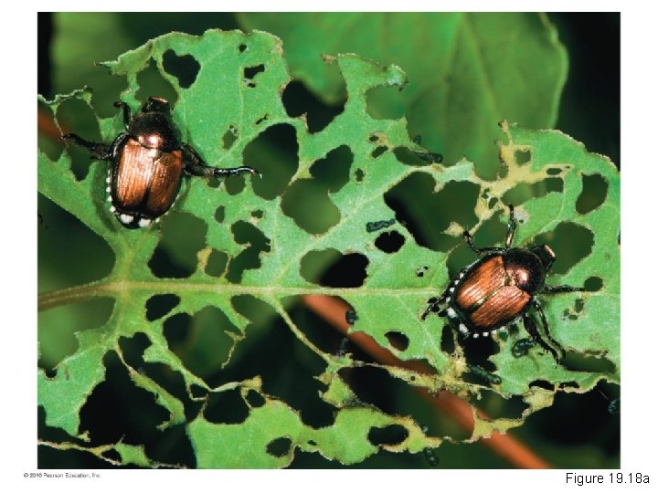
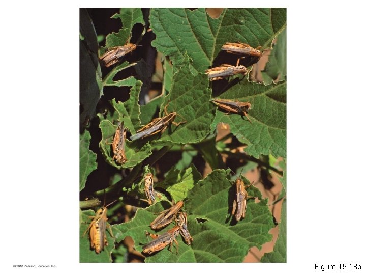
Integrated Pest Management • Agricultural operations create their own highly managed ecosystems that – Have genetically similar individuals (a monoculture) – Are planted in close proximity to each other – Function as a “banquet” for – Plant-eating animals – Pathogenic bacteria – Viruses © 2010 Pearson Education, Inc.

• Like invasive species, most crop pests – Have an opportunistic life history pattern – Can cause extensive crop damage © 2010 Pearson Education, Inc.

Figure 19. 18

Figure 19. 18 a

Figure 19. 18 b

• Pesticides may – Result in pesticide-resistant pests – Kill the pest and their natural predators – Kill pollinators © 2010 Pearson Education, Inc.

• Integrated pest management (IPM) – Tolerates a low level of pests instead of total eradication – Produces a sustainable control of agricultural pests – Uses a combination of – Biological methods – Chemical methods – Cultural methods © 2010 Pearson Education, Inc.

• IPM methods include – Using pest-resistant varieties of crops – Using mixed-species plantings – Rotating crops to deprive the pest of a dependable food source © 2010 Pearson Education, Inc.

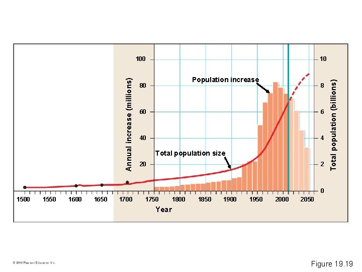
HUMAN POPULATION GROWTH The History of Human Population Growth • From 2000 to 500 years ago (in 1500) – Mortality was high – Births and deaths were about equal – The world population held steady at about 300 million © 2010 Pearson Education, Inc.

• The world’s population began to grow exponentially in the 1900 s due to advances in – Nutrition – Sanitation – Health care Blast Animation: Population Dynamics © 2010 Pearson Education, Inc.

10 Population increase 80 8 60 6 40 4 Total population size 20 2 Total population (billions) Annual increase (millions) 100 0 1500 1550 1600 1650 1700 1750 1800 1850 1900 1950 2000 2050 Year Figure 19. 19

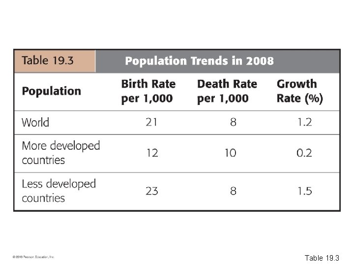
• Worldwide population growth rates reflect a mosaic of the changes occurring in different countries. – In the most developed nations, the overall growth rates are near zero. – In the developing world – Death rates have dropped – High birth rates persist © 2010 Pearson Education, Inc.

Table 19. 3

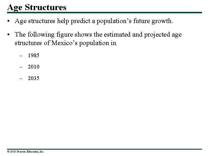
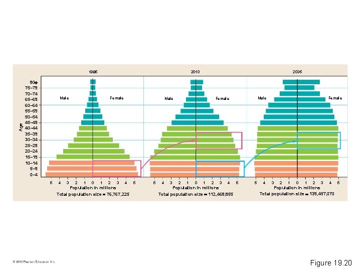
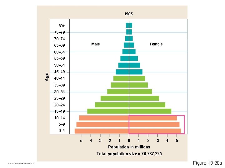
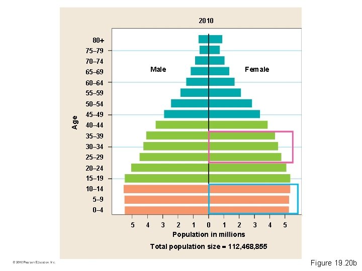
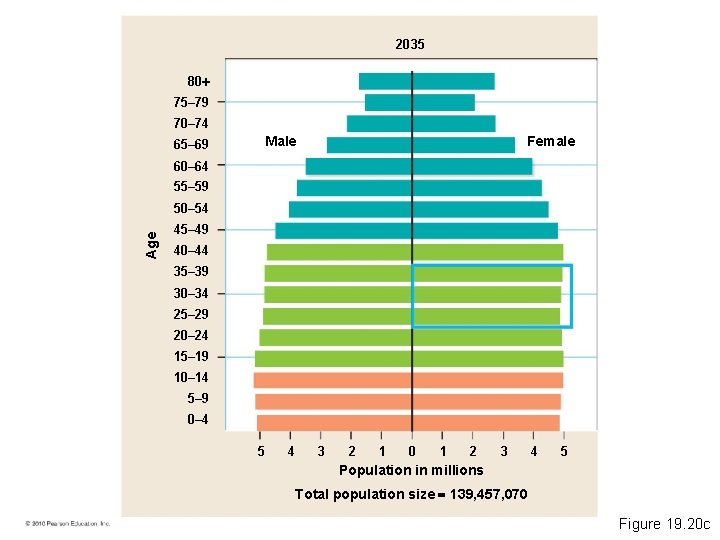
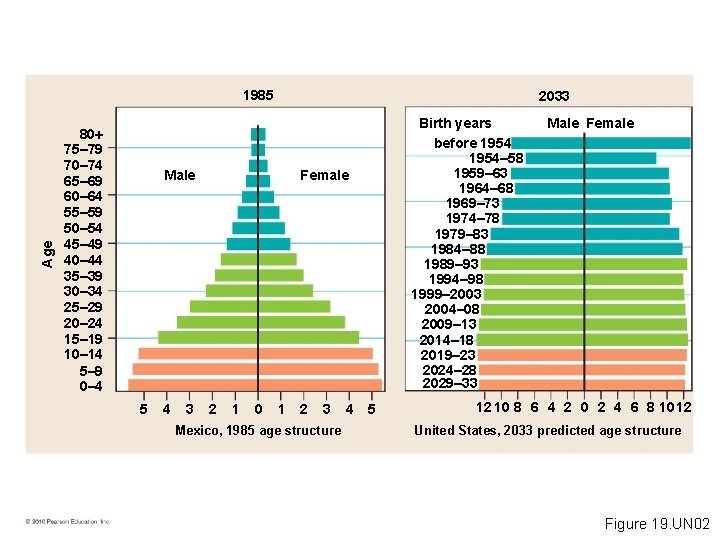
Age Structures • Age structures help predict a population’s future growth. • The following figure shows the estimated and projected age structures of Mexico’s population in – 1985 – 2010 – 2035 © 2010 Pearson Education, Inc.

Age 1985 80 75– 79 70– 74 65– 69 60– 64 55– 59 50– 54 45– 49 40– 44 35– 39 30– 34 25– 29 20– 24 15– 19 10– 14 5– 9 0– 4 2010 Male 5 4 3 Female 2 1 0 1 2 3 2035 Male 4 Population in millions Total population size 76, 767, 225 5 5 4 3 Male Female 2 1 0 1 2 3 4 Population in millions Total population size 112, 468, 855 5 5 4 Female 3 2 1 0 1 2 3 4 5 Population in millions Total population size 139, 457, 070 Figure 19. 20

1985 80 75– 79 70– 74 Male 65– 69 Female 60– 64 55– 59 Age 50– 54 45– 49 40– 44 35– 39 30– 34 25– 29 20– 24 15– 19 10– 14 5– 9 0– 4 5 4 3 2 1 0 1 2 3 4 5 Population in millions Total population size 76, 767, 225 Figure 19. 20 a

2010 80 75– 79 70– 74 Female Male 65– 69 60– 64 55– 59 Age 50– 54 45– 49 40– 44 35– 39 30– 34 25– 29 20– 24 15– 19 10– 14 5– 9 0– 4 5 4 3 2 1 0 1 2 3 4 5 Population in millions Total population size 112, 468, 855 Figure 19. 20 b

2035 80 75– 79 70– 74 Female Male 65– 69 60– 64 55– 59 Age 50– 54 45– 49 40– 44 35– 39 30– 34 25– 29 20– 24 15– 19 10– 14 5– 9 0– 4 5 4 3 2 1 0 1 2 3 4 5 Population in millions Total population size 139, 457, 070 Figure 19. 20 c

• Population momentum is the continuation of population growth as girls in the prereproductive age group reach their reproductive years. © 2010 Pearson Education, Inc.

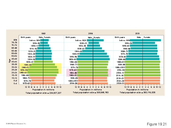
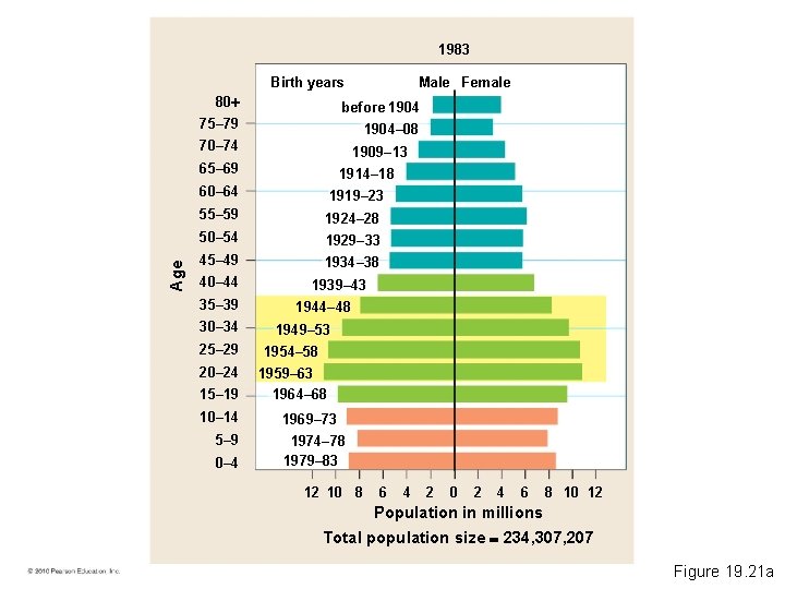
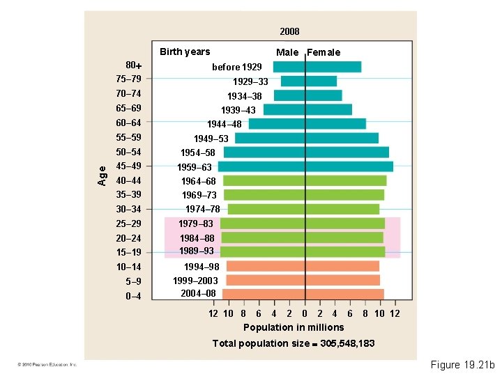
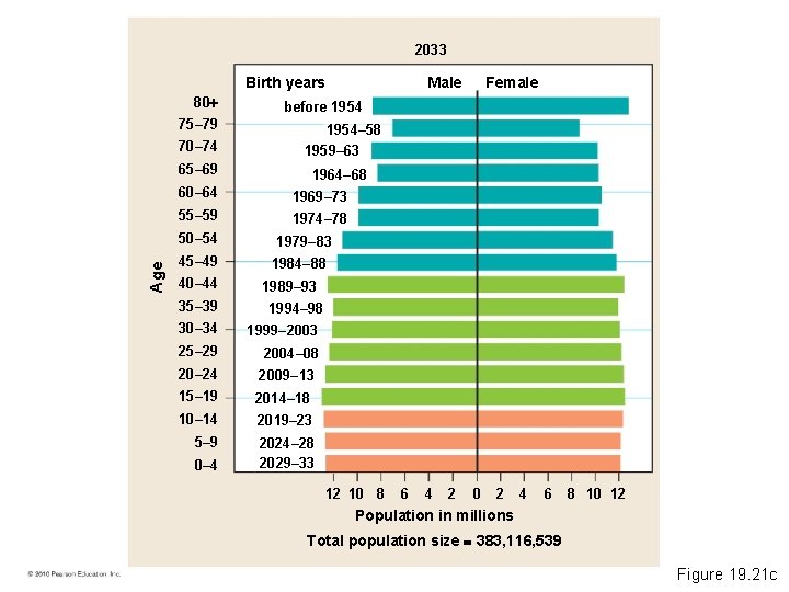
• Age structure diagrams may also indicate social conditions. An expanding population needs – Schools – Employment – Infrastructure • Trends in the age structure of the United States from 1983 to 2033 reveal important patterns. © 2010 Pearson Education, Inc.

2008 1983 Age Birth years 80 75– 79 70– 74 65– 69 60– 64 55– 59 50– 54 45– 49 40– 44 35– 39 30– 34 25– 29 20– 24 15– 19 10– 14 5– 9 0– 4 Male Female Birth years before 1904– 08 1909– 13 1914– 18 1919– 23 1924– 28 1929– 33 1934– 38 1939– 43 1944– 48 1949– 53 1954– 58 1959– 63 1964– 68 2033 Birth years Male Female 1969– 73 1974– 78 1979– 83 1994– 98 1999– 2003 2004– 08 12 10 8 6 4 2 0 2 4 6 8 10 12 Population in millions Total population size 234, 307, 207 12 10 8 6 4 2 0 2 4 Male Female before 1954– 58 1959– 63 1964– 68 1969– 73 1974– 78 1979– 83 1984– 88 1989– 93 1994– 98 1999– 2003 2004– 08 2009– 13 2014– 18 2019– 23 2024– 28 2029– 33 before 1929– 33 1934– 38 1939– 43 1944– 48 1949– 53 1954– 58 1959– 63 1964– 68 1969– 73 1974– 78 1979– 83 1984– 88 1989– 93 6 8 10 12 Population in millions Total population size 305, 548, 183 12 10 8 6 4 2 0 2 4 6 8 10 12 Population in millions Total population size 383, 116, 539 Figure 19. 21

1983 Birth years 80 before 1904 75– 79 1904– 08 70– 74 1909– 13 65– 69 Age Male Female 1914– 18 60– 64 1919– 23 55– 59 1924– 28 50– 54 1929– 33 45– 49 1934– 38 40– 44 35– 39 30– 34 1939– 43 1944– 48 1949– 53 25– 29 1954– 58 20– 24 1959– 63 1964– 68 15– 19 10– 14 5– 9 0– 4 1969– 73 1974– 78 1979– 83 12 10 8 6 4 2 0 2 4 6 8 10 12 Population in millions Total population size 234, 307, 207 Figure 19. 21 a

2008 Birth years 80 Male Female before 1929 75– 79 1929– 33 70– 74 1934– 38 65– 69 60– 64 55– 59 Age 50– 54 45– 49 1939– 43 1944– 48 1949– 53 1954– 58 1959– 63 40– 44 1964– 68 35– 39 1969– 73 30– 34 1974– 78 25– 29 1979– 83 20– 24 1984– 88 1989– 93 15– 19 10– 14 1994– 98 5– 9 1999– 2003 2004– 08 0– 4 12 10 8 6 4 2 0 2 4 6 8 10 12 Population in millions Total population size 305, 548, 183 Figure 19. 21 b

2033 Birth years 80 1954– 58 1959– 63 65– 69 Age 1964– 68 60– 64 1969– 73 55– 59 1974– 78 50– 54 45– 49 40– 44 35– 39 1979– 83 1984– 88 1989– 93 1994– 98 30– 34 1999– 2003 25– 29 2004– 08 20– 24 2009– 13 15– 19 2014– 18 10– 14 2019– 23 5– 9 2024– 28 2029– 33 0– 4 Female before 1954 75– 79 70– 74 Male 12 10 8 6 4 2 0 2 4 6 8 10 12 Population in millions Total population size 383, 116, 539 Figure 19. 21 c

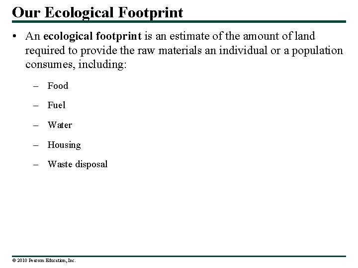
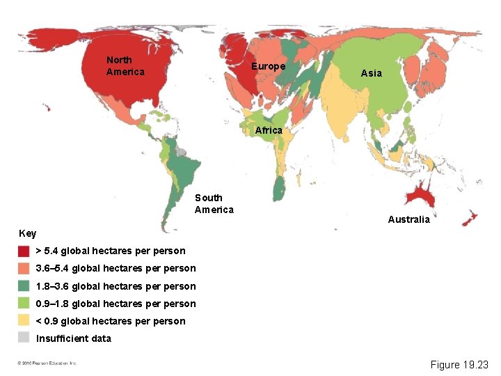
Our Ecological Footprint • An ecological footprint is an estimate of the amount of land required to provide the raw materials an individual or a population consumes, including: – Food – Fuel – Water – Housing – Waste disposal © 2010 Pearson Education, Inc.

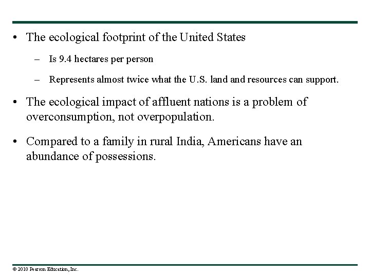
• The ecological footprint of the United States – Is 9. 4 hectares person – Represents almost twice what the U. S. land resources can support. • The ecological impact of affluent nations is a problem of overconsumption, not overpopulation. • Compared to a family in rural India, Americans have an abundance of possessions. © 2010 Pearson Education, Inc.

Figure 19. 22

Figure 19. 22 a

Figure 19. 22 b

• There is tremendous disparity in consumption throughout the world. • The world’s richest countries – Have 20% of the global population – Use 86% of the world’s resources • The rest of the world – Has 80% of the population – Uses just 14% of global resources © 2010 Pearson Education, Inc.

North America Europe Asia Africa South America Australia Key > 5. 4 global hectares person 3. 6– 5. 4 global hectares person 1. 8– 3. 6 global hectares person 0. 9– 1. 8 global hectares person < 0. 9 global hectares person Insufficient data Figure 19. 23

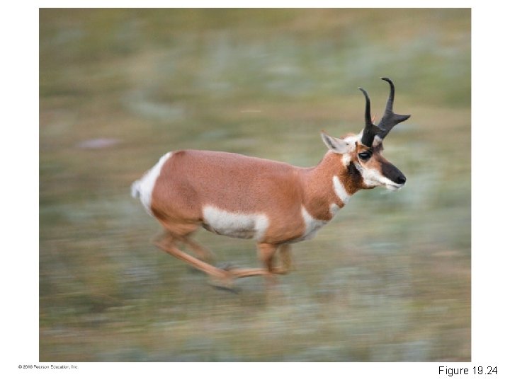
Evolution Connection: Humans as an Invasive Species • Pronghorn antelope – Roamed the open plains and shrub deserts of North America millions of years ago – Have a top speed of 97 km/h (60 mph) – Are the fastest mammal on the continent • Pronghorn speed is likely an adaptation to outrun American cheetahs, which went extinct about 10, 000 years ago. © 2010 Pearson Education, Inc.

Figure 19. 24

• About 10, 000 years ago – Changes in the biotic and abiotic environments happened too rapidly for an evolutionary response – Many large North American mammals, in addition to American cheetahs, went extinct, including – Lions – Saber-toothed cats – Towering short-faced bears © 2010 Pearson Education, Inc.

• Although still hotly disputed, many scientists think that the extinction at the end of the ice age about 10, 000 years ago was in part the result of the human invasion of North America, with humans serving as the damaging invasive species. © 2010 Pearson Education, Inc.

• Like other invasive species, humans may change the environment at an accelerating pace and too rapidly for other species to evolve and survive. © 2010 Pearson Education, Inc.

Percentage of survivors (log scale) 100 Type I: most individuals survive to older age intervals I 10 Type II: survivorship constant over life span II 1 Type III: low survivorship at early age intervals III 0. 1 0 50 100 Percentage of maximum life span Figure 19. UN 01

Age 1985 80 75– 79 70– 74 65– 69 60– 64 55– 59 50– 54 45– 49 40– 44 35– 39 30– 34 25– 29 20– 24 15– 19 10– 14 5– 9 0– 4 2033 Male 5 4 3 Birth years before 1954– 58 1959– 63 1964– 68 1969– 73 1974– 78 1979– 83 1984– 88 1989– 93 1994– 98 1999– 2003 2004– 08 2009– 13 2014– 18 2019– 23 2024– 28 2029– 33 Female 2 1 0 1 2 3 Mexico, 1985 age structure 4 5 Male Female 12 10 8 6 4 2 0 2 4 6 8 1012 United States, 2033 predicted age structure Figure 19. UN 02

0 Figure 19. UN 03