Chapter 19 Numerical Differentiation Estimate the derivatives slope

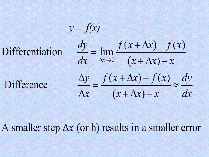
Chapter 19 Numerical Differentiation § Estimate the derivatives (slope, curvature, etc. ) of a function by using the function values at only a set of discrete points § Ordinary differential equation (ODE) § Partial differential equation (PDE) § Represent the function by Taylor polynomials or Lagrange interpolation § Evaluate the derivatives of the interpolation polynomial at selected (unevenly distributed) nodal points

Evenly distributed points along the x-axis xi-3 xi-2 xi-1 xi xi+1 xi+2 xi+3 Distance between two neighboring points is the same, i. e. h. Unevenly distributed points along the x-axis x 1 x 2 x 3

Numerical Differentiation Forward difference Backward difference Centered difference

Forward difference ue r T i r e d iv t a v e on i t a m i x Appro h xi 1 xi xi+1 x

Backward difference e A pp ro xi m at io n ue r T i r e d iv t a v h xi 1 xi xi+1 x

Centered difference ue r T i r e d iv t a v e n o i t a m i x o r p p A 2 h xi 1 xi xi+1 x

y First Derivatives i-2 i-1 § Forward difference § Backward difference § Central difference i i+1 i+2 x

Truncation Errors § Uniform grid spacing

Example: First Derivatives § Use forward and backward difference approximations to estimate the first derivative of at x = 0. 5 with h = 0. 5 and 0. 25 (exact sol. = -0. 9125) § Forward Difference § Backward Difference

Example: First Derivative § Use central difference approximation to estimate the first derivative of at x = 0. 5 with h = 0. 5 and 0. 25 (exact sol. = -0. 9125) § Central Difference

Second-Derivatives § Taylor-series expansion § Uniform grid spacing § Second-order accurate O(h 2)

Centered Finite-Divided Differences

Forward Finite-divided differences

Backward finite-divided differences

First Derivatives Parabolic curve i-2 i-1 i § 3 -point Forward difference § 3 -point Backward difference i+1 i+2

Example: First Derivatives § Use forward and backward difference approximations of O(h 2) to estimate the first derivative of at x = 0. 5 with h = 0. 25 (exact sol. = -0. 9125) § Forward Difference § Backward Difference

Higher Derivatives § All second-order accurate O(h 2) § More nodal points are needed for higher derivatives § Higher order formula may be derived

19. 3 Richardson Extrapolation D is the true value but unknown and D(h 1) is an approximation based on the step size h 1. Reducing the step size to half, h 2 =h 1/2, we obtained another approximation D(h 2). By properly combining the two approximations, D(h 1) & D(h 2), the error is reduced to O(h 4).

Example of using Richardson Extrapolation Central Difference Scheme By combining the two approximations, D(h/2) & D(h), the error of f’(h) is reduced to O(h 4).

Ex 19. 2: Richardson Extrapolation § Use central difference approximation to estimate the first derivative of at x = 0. 5 with h = 0. 5 and 0. 25 (exact sol. = -0. 9125)

General Three-Point Formula Ø Lagrange interpolation polynomial for unequally spaced data

Lagrange Interpolation § 1 st-order Lagrange polynomial § Second-order Lagrange polynomial

Lagrange Interpolation § Third-order Lagrange polynomial

Lagrange Interpolation L 2(x)f(x 2) L 0(x)f(x 0) x 0 L 1(x)f(x 1) x 1 x 2

General Three-Point Formula Ø Lagrange interpolation polynomial for unequally spaced data Ø First derivative

Second Derivative § First Derivative for unequally spaced data § Second Derivative for unequally spaced data

Differentiation of Noisy Data

MATLAB’s Methods § Derivatives are sensitive to the noise § Use least square fit before taking derivatives § p = polyfit(x, y, n) - coefficients of Pn(x) § polyfit(p, x) - evaluation of Pn(x) § polyder(p) - differentiation