Chapter 18 Portfolio Performance Evaluation Mc GrawHillIrwin Copyright

Chapter 18 Portfolio Performance Evaluation Mc. Graw-Hill/Irwin Copyright © 2010 by The Mc. Graw-Hill Companies, Inc. All rights reserved.

18. 1 Risk-Adjusted Returns 18 -2

Types of management revisited • Passive management 1. Capital allocation between cash and the risky portfolio 2. Asset allocation within the risky portfolio. – How passive the management actually is varies • “Set it and forget it” • Change allocations in 1 or 2 according to perceptions of risk to keep current with portfolio goals. • Active management – Forecasting future rates of return on either/both asset classes and individual securities 18 -3

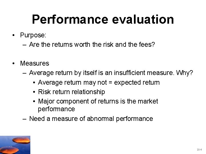
Performance evaluation • Purpose: – Are the returns worth the risk and the fees? • Measures – Average return by itself is an insufficient measure. Why? • Average return may not = expected return • Risk return relationship • Major component of returns is the market performance – Need a measure of abnormal performance 18 -4

Abnormal Performance How is abnormal performance measured? Comparisons to peer groups Rank fund performance within a given category Benchmark portfolio such as an index Really need measures that consider risk: Calculate reward to risk measures such as the alpha, Sharpe Measure (or variations) 18 -5

Factors That Lead to Abnormal Performance • Successful across asset allocations • Superior allocation within each asset class – Sectors or industries • Overweight better performing sectors, underweight poorer performers • Individual security selection • Pick the right stocks, those with performance better than expected 18 -6

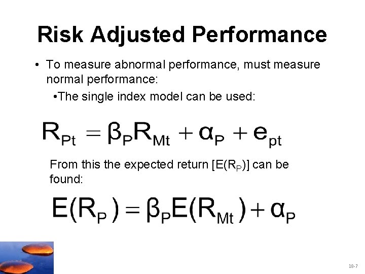
Risk Adjusted Performance • To measure abnormal performance, must measure normal performance: • The single index model can be used: From this the expected return [E(RP)] can be found: 18 -7

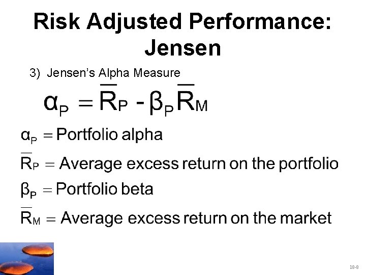
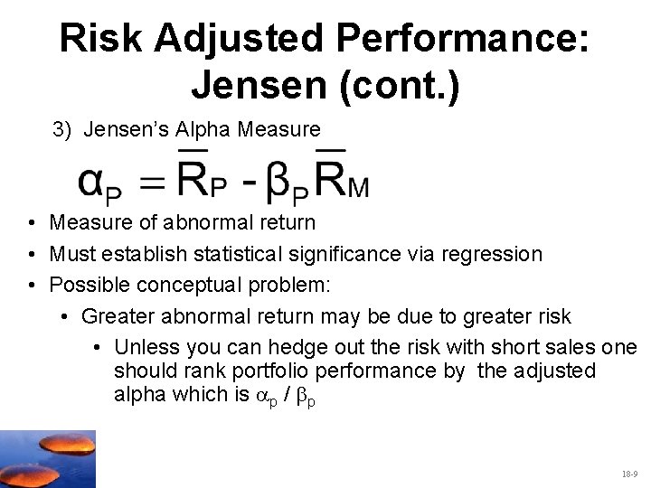
Risk Adjusted Performance: Jensen 3) Jensen’s Alpha Measure 18 -8

Risk Adjusted Performance: Jensen (cont. ) 3) Jensen’s Alpha Measure • Measure of abnormal return • Must establish statistical significance via regression • Possible conceptual problem: • Greater abnormal return may be due to greater risk • Unless you can hedge out the risk with short sales one should rank portfolio performance by the adjusted alpha which is p / p 18 -9

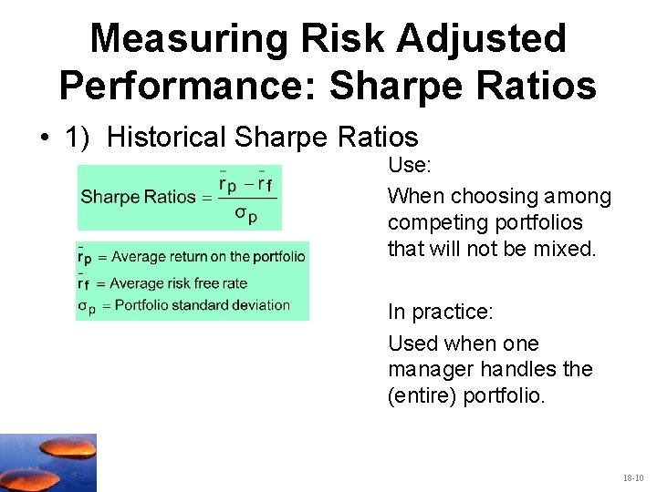
Measuring Risk Adjusted Performance: Sharpe Ratios • 1) Historical Sharpe Ratios Use: When choosing among competing portfolios that will not be mixed. In practice: Used when one manager handles the (entire) portfolio. 18 -10

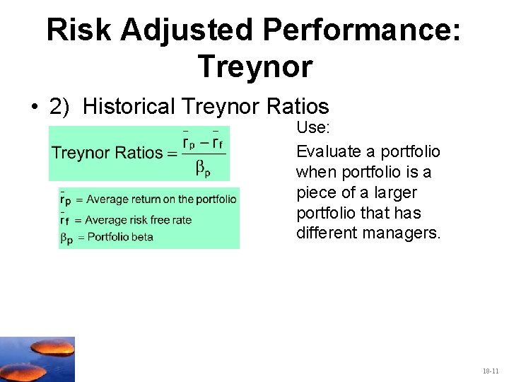
Risk Adjusted Performance: Treynor • 2) Historical Treynor Ratios Use: Evaluate a portfolio when portfolio is a piece of a larger portfolio that has different managers. 18 -11

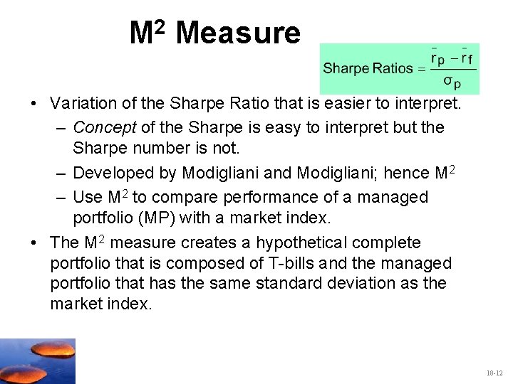
M 2 Measure • Variation of the Sharpe Ratio that is easier to interpret. – Concept of the Sharpe is easy to interpret but the Sharpe number is not. – Developed by Modigliani and Modigliani; hence M 2 – Use M 2 to compare performance of a managed portfolio (MP) with a market index. • The M 2 measure creates a hypothetical complete portfolio that is composed of T-bills and the managed portfolio that has the same standard deviation as the market index. 18 -12

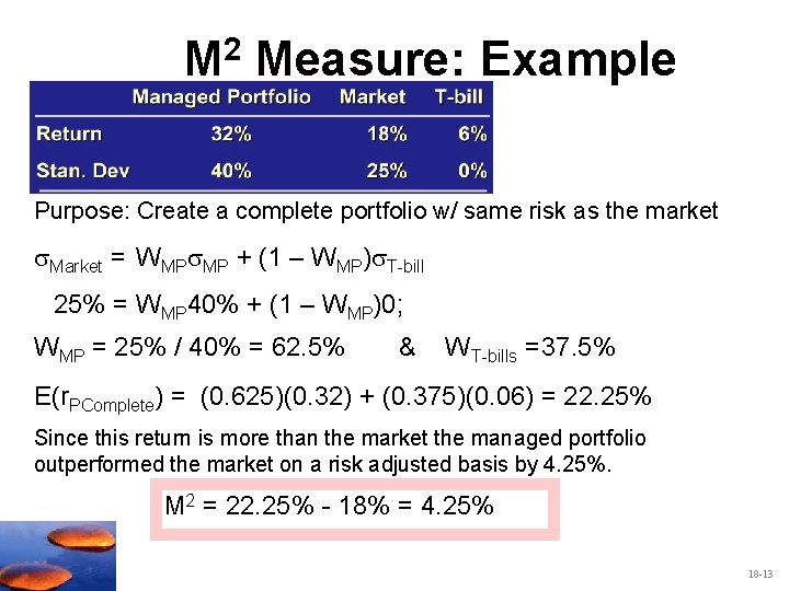
2 M Measure: Example Purpose: Create a complete portfolio w/ same risk as the market Market = WMP MP + (1 – WMP) T-bill 25% = WMP 40% + (1 – WMP)0; 25% / 40% = 62. 5% 37. 5% WMP = & W T-bills = E(r. PComplete) = (0. 625)(0. 32) + (0. 375)(0. 06) = 22. 25% Since this return is more than the market the managed portfolio outperformed the market on a risk adjusted basis by 4. 25%. M 2 = 22. 25% - 18% = 4. 25% 18 -13

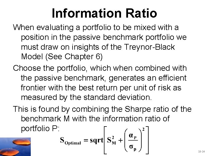
Information Ratio When evaluating a portfolio to be mixed with a position in the passive benchmark portfolio we must draw on insights of the Treynor-Black Model (See Chapter 6) Choose the portfolio, which when combined with the passive benchmark, generates an efficient frontier with the best return per unit of risk as measured by the standard deviation. This is found by combining the Sharpe ratio of the benchmark M with the information ratio of portfolio P: 18 -14

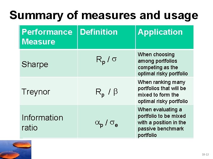
Summary of measures and usage Performance Definition Measure Sharpe Treynor Information ratio Rp / Application When choosing among portfolios competing as the optimal risky portfolio Rp / When ranking many portfolios that will be mixed to form the optimal risky portfolio p / e When evaluating a portfolio to be mixed with a position in the passive benchmark portfolio 18 -15

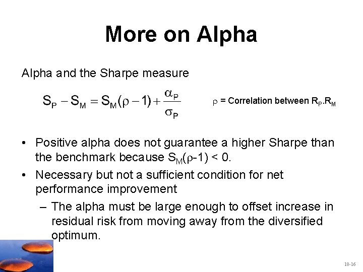
More on Alpha and the Sharpe measure = Correlation between RP. RM • Positive alpha does not guarantee a higher Sharpe than the benchmark because SM( -1) < 0. • Necessary but not a sufficient condition for net performance improvement – The alpha must be large enough to offset increase in residual risk from moving away from the diversified optimum. 18 -16

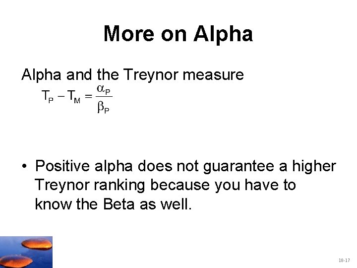
More on Alpha and the Treynor measure • Positive alpha does not guarantee a higher Treynor ranking because you have to know the Beta as well. 18 -17

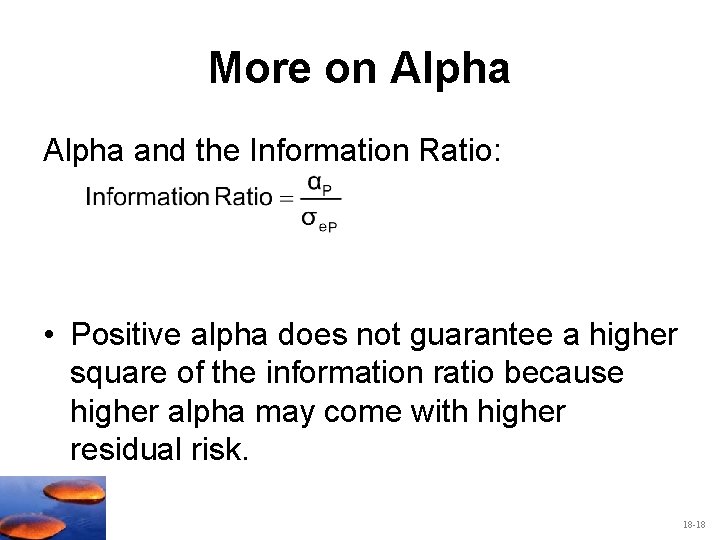
More on Alpha and the Information Ratio: • Positive alpha does not guarantee a higher square of the information ratio because higher alpha may come with higher residual risk. 18 -18

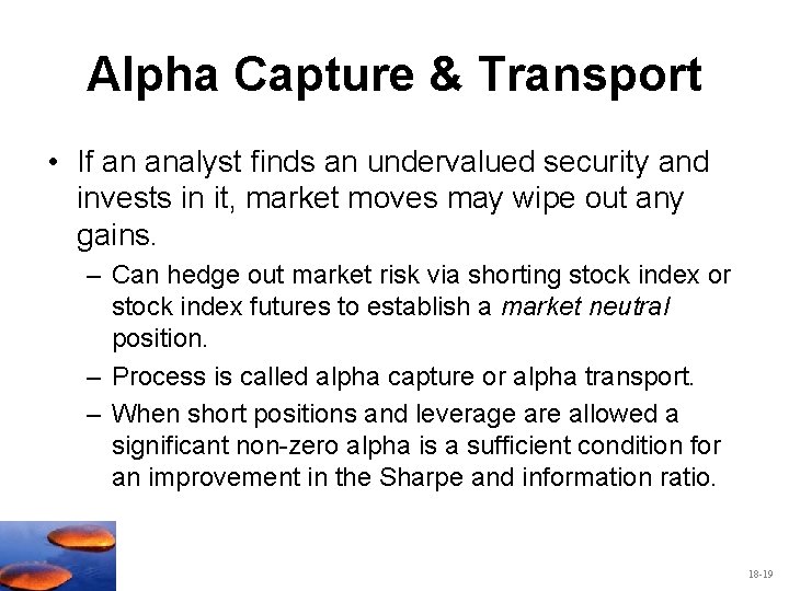
Alpha Capture & Transport • If an analyst finds an undervalued security and invests in it, market moves may wipe out any gains. – Can hedge out market risk via shorting stock index or stock index futures to establish a market neutral position. – Process is called alpha capture or alpha transport. – When short positions and leverage are allowed a significant non-zero alpha is a sufficient condition for an improvement in the Sharpe and information ratio. 18 -19

Performance measures for P, Q, M & cash 18 -20

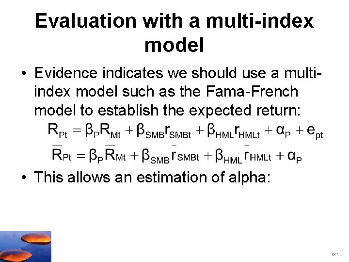
Evaluation with a multi-index model • Evidence indicates we should use a multiindex model such as the Fama-French model to establish the expected return: • This allows an estimation of alpha: 18 -21

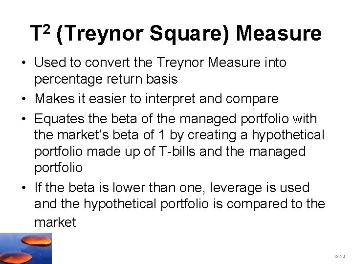
T 2 (Treynor Square) Measure • Used to convert the Treynor Measure into percentage return basis • Makes it easier to interpret and compare • Equates the beta of the managed portfolio with the market’s beta of 1 by creating a hypothetical portfolio made up of T-bills and the managed portfolio • If the beta is lower than one, leverage is used and the hypothetical portfolio is compared to the market 18 -22

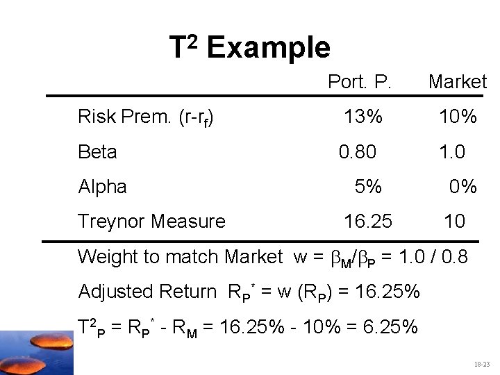
T 2 Example Port. P. Market 13% 10% 0. 80 1. 0 Alpha 5% 0% Treynor Measure 16. 25 10 Risk Prem. (r-rf) Beta Weight to match Market w = M/ P = 1. 0 / 0. 8 Adjusted Return RP* = w (RP) = 16. 25% T 2 P = RP* - RM = 16. 25% - 10% = 6. 25% 18 -23

18. 2 Style Analysis 18 -24

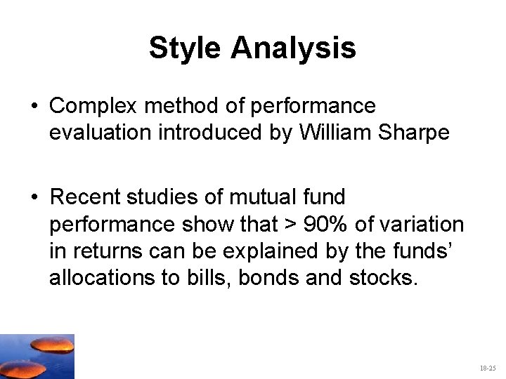
Style Analysis • Complex method of performance evaluation introduced by William Sharpe • Recent studies of mutual fund performance show that > 90% of variation in returns can be explained by the funds’ allocations to bills, bonds and stocks. 18 -25

Style Analysis • Explaining percentage returns by allocation to style • Style Analysis has become popular with the industry 18 -26

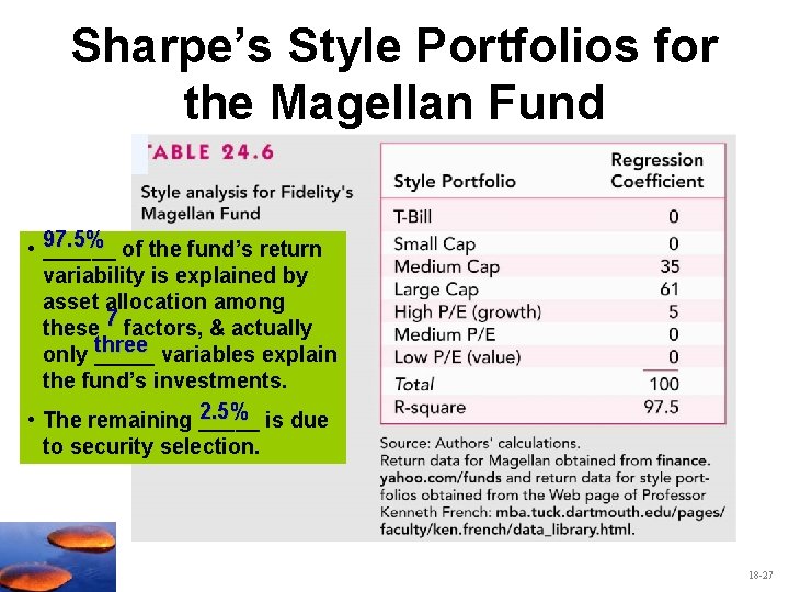
Sharpe’s Style Portfolios for the Magellan Fund • 97. 5% ______ of the fund’s return variability is explained by asset allocation among 7 these factors, & actually three only _____ variables explain the fund’s investments. 2. 5% • The remaining _____ is due to security selection. 18 -27

18. 3 Morningstar’s Risk-Adjusted Ratings 18 -28

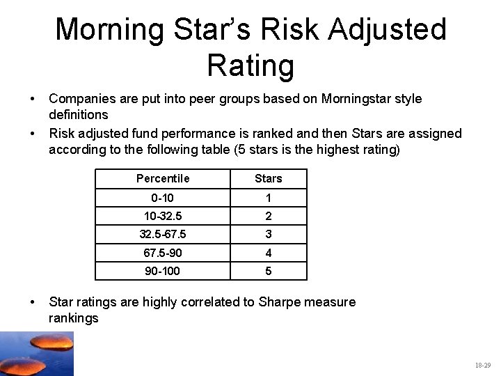
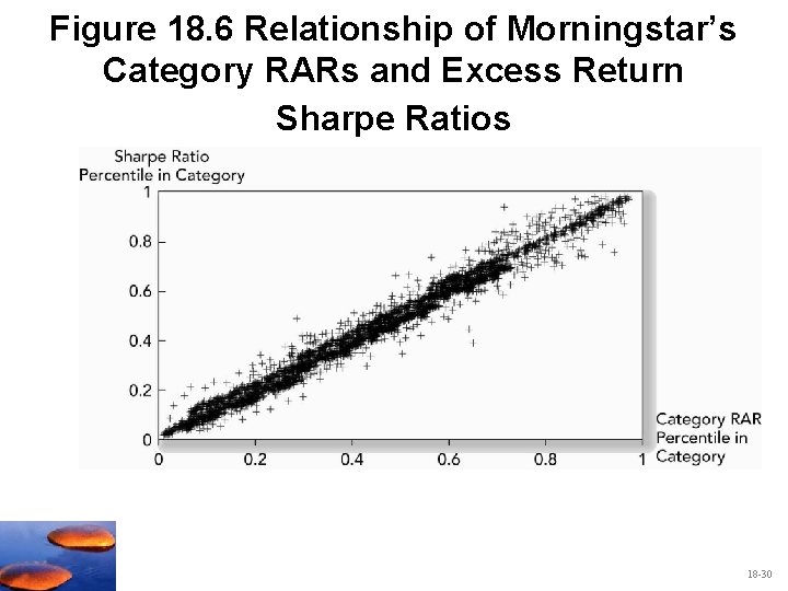
Morning Star’s Risk Adjusted Rating • • • Companies are put into peer groups based on Morningstar style definitions Risk adjusted fund performance is ranked and then Stars are assigned according to the following table (5 stars is the highest rating) Percentile Stars 0 -10 1 10 -32. 5 2 32. 5 -67. 5 3 67. 5 -90 4 90 -100 5 Star ratings are highly correlated to Sharpe measure rankings 18 -29

Figure 18. 6 Relationship of Morningstar’s Category RARs and Excess Return Sharpe Ratios 18 -30

18. 4 Risk Adjustment With Changing Portfolio Composition 18 -31

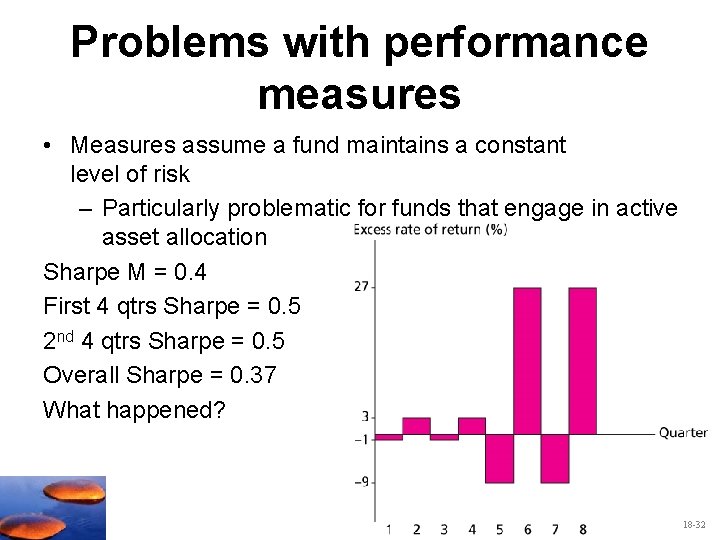
Problems with performance measures • Measures assume a fund maintains a constant level of risk – Particularly problematic for funds that engage in active asset allocation Sharpe M = 0. 4 First 4 qtrs Sharpe = 0. 5 2 nd 4 qtrs Sharpe = 0. 5 Overall Sharpe = 0. 37 What happened? 18 -32

Problems with performance measures • In a large universe of funds, some funds will have abnormal performance in every period just by chance. – Requires statistical work • Volatility is quite high and creates large errors in estimation 18 -33

18. 5 Performance Attribution Procedures 18 -34

Performance Attribution • Decomposing overall performance into components • Performance is determined by specific portfolio choices, • Major performance determinants: – Broad asset allocation among types of securities, – Industry weighting in equity portfolio, – Security choice, – Timing of purchases and sales. 18 -35

Process of Attributing Performance to Components • Set up a benchmark or ‘bogey’ portfolio • Use indexes for each component in the bogey • Use target weight structure in the bogey 18 -36

Process of Attributing Performance to Components • Calculate the return on the ‘bogey’ and on the managed portfolio • Explain the difference in return based on component weights or selection • Summarize the performance differences into appropriate categories 18 -37

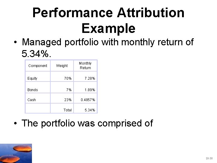
Performance Attribution Example • Managed portfolio with monthly return of 5. 34%. Component Weight Monthly Return Equity 70% 7. 28% Bonds 7% 1. 89% Cash 23% 0. 4857% Total 5. 34% • The portfolio was comprised of 18 -38

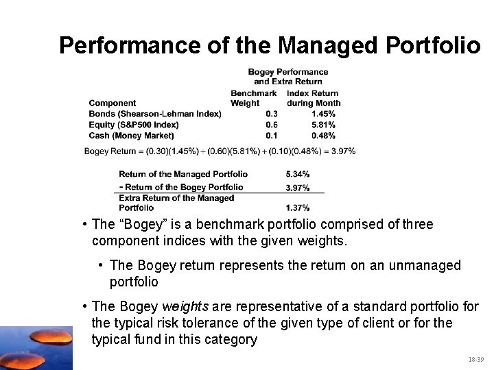
Performance of the Managed Portfolio • The “Bogey” is a benchmark portfolio comprised of three component indices with the given weights. • The Bogey return represents the return on an unmanaged portfolio • The Bogey weights are representative of a standard portfolio for the typical risk tolerance of the given type of client or for the typical fund in this category 18 -39

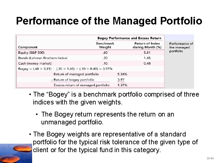
Performance of the Managed Portfolio • The “Bogey” is a benchmark portfolio comprised of three indices with the given weights. • The Bogey return represents the return on an unmanaged portfolio. • The Bogey weights are representative of a standard portfolio for the typical risk tolerance of the given type of client or for the typical fund in this category. 18 -40

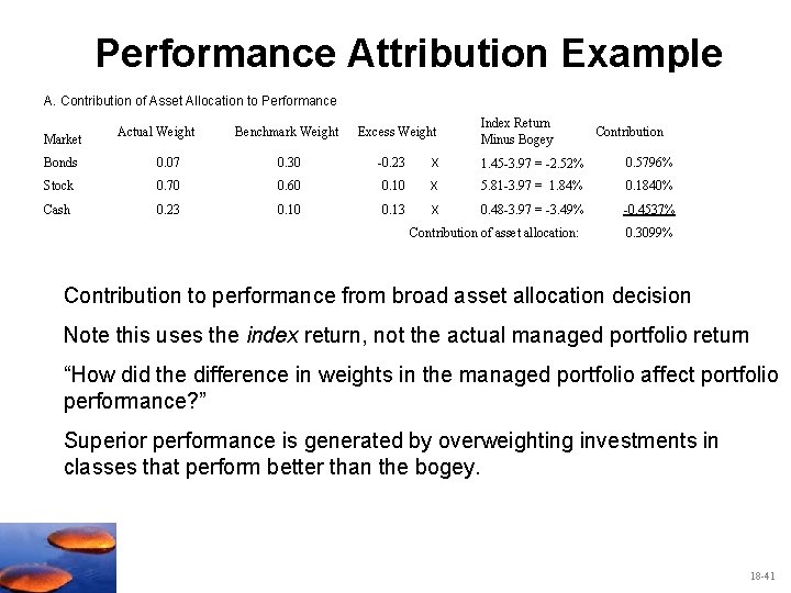
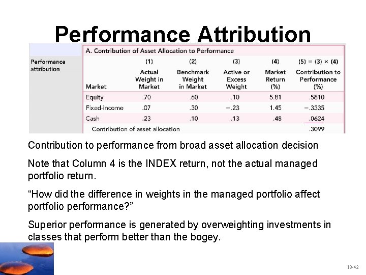
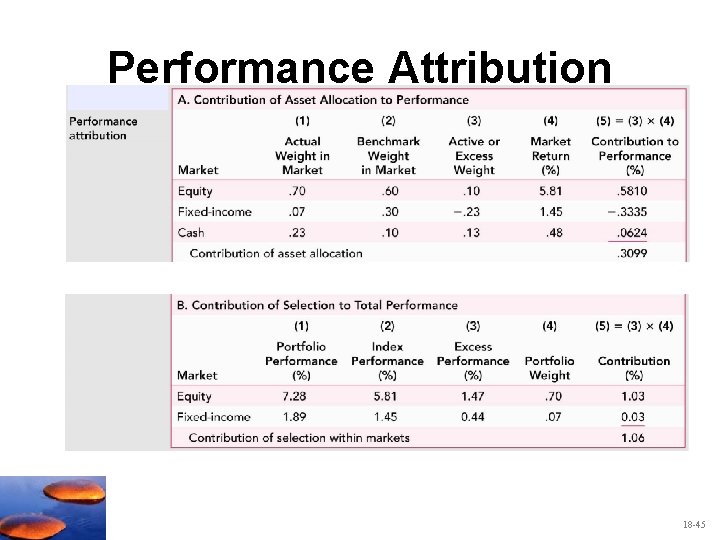
Performance Attribution Example A. Contribution of Asset Allocation to Performance Market Actual Weight Benchmark Weight Bonds 0. 07 0. 30 Stock 0. 70 0. 60 Cash 0. 23 0. 10 Excess Weight Index Return Minus Bogey x 1. 45 -3. 97 = -2. 52% = x 0. 10 5. 81 -3. 97 = 1. 84% = 0. 13 0. 48 -3. 97 = -3. 49% x = Contribution of asset allocation: -0. 23 Contribution 0. 5796% 0. 1840% -0. 4537% 0. 3099% Contribution to performance from broad asset allocation decision Note this uses the index return, not the actual managed portfolio return “How did the difference in weights in the managed portfolio affect portfolio performance? ” Superior performance is generated by overweighting investments in classes that perform better than the bogey. 18 -41

Performance Attribution Contribution to performance from broad asset allocation decision Note that Column 4 is the INDEX return, not the actual managed portfolio return. “How did the difference in weights in the managed portfolio affect portfolio performance? ” Superior performance is generated by overweighting investments in classes that perform better than the bogey. 18 -42

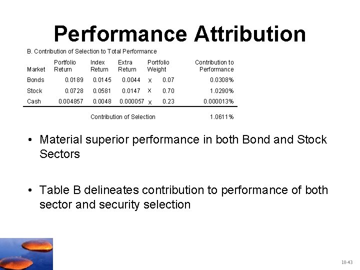
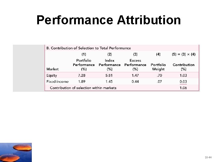
Performance Attribution B. Contribution of Selection to Total Performance Market Portfolio Return Index Return Extra Return Portfolio Weight Contribution to Performance x x 0. 07 0. 0308% 0. 70 1. 0290% 0. 000057 x 0. 23 0. 000013% Bonds 0. 0189 0. 0145 0. 0044 Stock 0. 0728 0. 0581 0. 0147 Cash 0. 004857 0. 0048 Contribution of Selection 1. 0611% • Material superior performance in both Bond and Stock Sectors • Table B delineates contribution to performance of both sector and security selection 18 -43

Performance Attribution 18 -44

Performance Attribution 18 -45

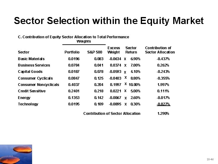
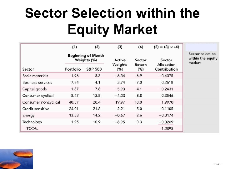
Sector Selection within the Equity Market C. Contribution of Equity Sector Allocation to Total Performance Weights Sector Portfolio S&P 500 Excess Weight Sector Return Contribution of Sector Allocation Basic Materials 0. 0196 0. 083 -0. 0634 x 6. 90% -0. 437% Business Services 0. 0784 0. 041 0. 0374 x 7. 00% 0. 262% Capital Goods 0. 0187 0. 078 -0. 0593 x 4. 10% -0. 243% Consumer Cyclicals 0. 0847 0. 125 -0. 0403 x 8. 80% -0. 355% Consumer Noncyclicals 0. 4037 0. 204 0. 1997 x 10. 00% 1. 997% Credit Sensitive 0. 2401 0. 218 0. 0221 x 5. 00% 0. 111% Energy 0. 1353 0. 142 -0. 0067 x 2. 60% -0. 017% Technology 0. 0195 0. 109 -0. 0895 x 0. 30% -0. 027% Contribution of Sector Allocation 1. 290% 18 -46

Sector Selection within the Equity Market 18 -47

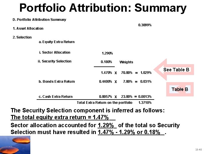
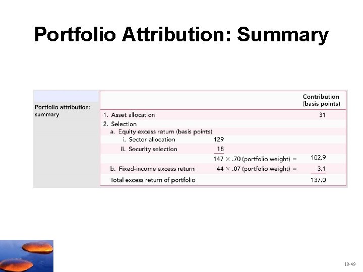
Portfolio Attribution: Summary D. Portfolio Attribution Summary 0. 3099% 1. Asset Allocation 2. Selection a. Equity Extra Return i. Sector Allocation 1. 290% ii. Security Selection 0. 180% b. Bonds Extra Return Weights 1. 470% x 70. 00% = 1. 029% 0. 4400% x 7. 00% = 0. 031% See Table B c. Cash Extra Return 0. 0057% x 23. 00% Total Extra Return on the portfolio = 0. 0013% 1. 3710% The Security Selection component is inferred as follows: _________________ The total equity extra return = 1. 47% 1. 29% Sector allocation accounted for ______ of the total so Security 1. 47% - 1. 29% or 0. 18% Selection must have resulted in ___________. 18 -48

Portfolio Attribution: Summary 18 -49

18. 6 Market Timing 18 -50

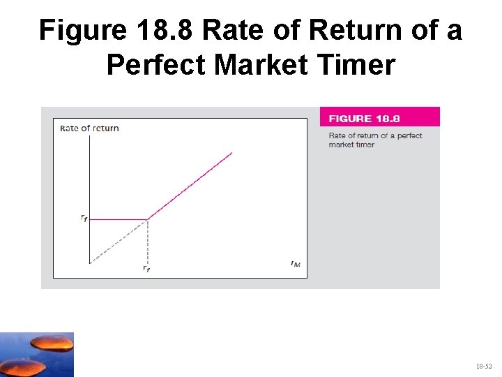
Market Timing • Adjust the asset allocation for movements in the market – Shift between stocks and money market instruments or bonds – With perfect ability to forecast behaves like an option – Little evidence of market timing ability 18 -51

Figure 18. 8 Rate of Return of a Perfect Market Timer 18 -52

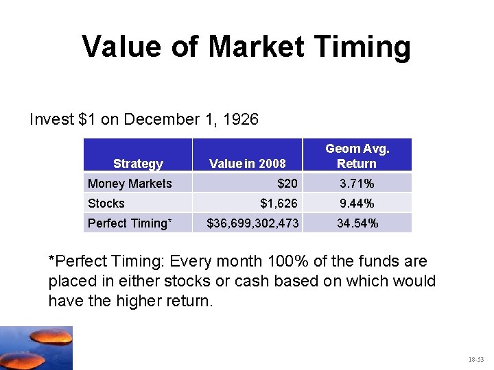
Value of Market Timing Invest $1 on December 1, 1926 Strategy Money Markets Stocks Perfect Timing* Value in 2008 Geom Avg. Return $20 3. 71% $1, 626 9. 44% $36, 699, 302, 473 34. 54% *Perfect Timing: Every month 100% of the funds are placed in either stocks or cash based on which would have the higher return. 18 -53

With Imperfect Ability to Forecast • Takes a long time horizon to judge the ability • Judge proportions of correct calls – Bull markets and bear market calls 18 -54

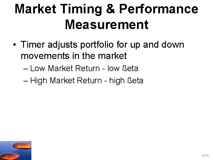
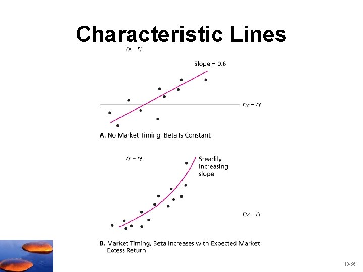
Market Timing & Performance Measurement • Timer adjusts portfolio for up and down movements in the market – Low Market Return - low ßeta – High Market Return - high ßeta 18 -55

Characteristic Lines 18 -56

Selected Problems 18 -57

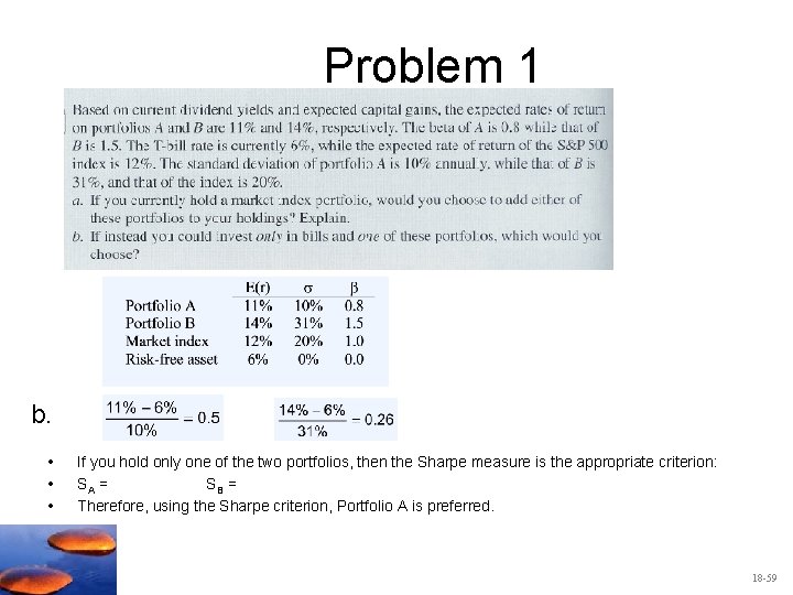
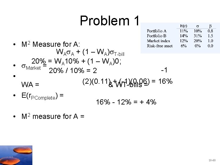
Problem 1 11% – [6% + 0. 8(12% – 6%)] = 0. 2% 14% – [6% + 1. 5(12% – 6%)] = – 1. 0% • The alphas for the two portfolios are: • a. A = • B = • Might add A if you believe the alpha is significant, might short B if you believe its alpha is significant, should check Treynor. 18 -58

Problem 1 b. • • • If you hold only one of the two portfolios, then the Sharpe measure is the appropriate criterion: SA = SB = Therefore, using the Sharpe criterion, Portfolio A is preferred. 18 -59

Problem 1 • M 2 Measure for A: WA A + (1 – WA) T-bill 20% = WA 10% + (1 – WA)0; • Market = -1 20% / 10% = 2 • (2)(0. 11) + (-1)(0. 06) = 16% WA = & WT-bills = • E(r. PComplete) = 16% - 12% = + 4% • M 2 measure for A = 18 -60

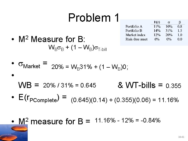
Problem 1 • M 2 Measure for B: WB B + (1 – WB) T-bill • Market = 20% = W 31% + (1 – W )0; B B • 20% / 31% = 0. 645 0. 355 WB = & WT-bills = • E(r. PComplete) = (0. 645)(0. 14) + (0. 355)(0. 06) = 11. 16% • M 2 measure for B = 11. 16% - 12% = -0. 84% 18 -61

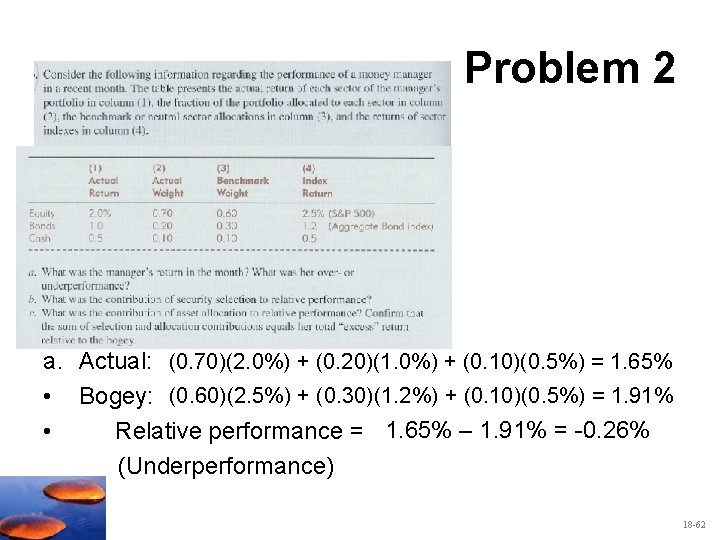
Problem 2 a. Actual: (0. 70)(2. 0%) + (0. 20)(1. 0%) + (0. 10)(0. 5%) = 1. 65% • Bogey: (0. 60)(2. 5%) + (0. 30)(1. 2%) + (0. 10)(0. 5%) = 1. 91% • Relative performance = 1. 65% – 1. 91% = -0. 26% (Underperformance) 18 -62

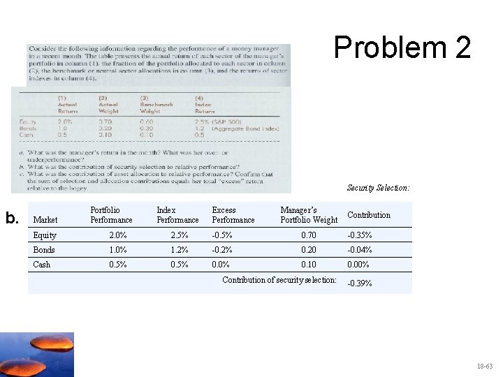
Problem 2 • Security Selection: b. Market Portfolio Performance Index Performance Excess Performance Manager’s Portfolio Weight Contribution Equity 2. 0% 2. 5% -0. 5% 0. 70 -0. 35% Bonds 1. 0% 1. 2% -0. 2% 0. 20 -0. 04% Cash 0. 5% 0. 0% 0. 10 0. 00% Contribution of security selection: -0. 39% 18 -63

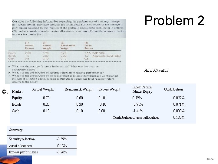
Problem 2 • Asset Allocation c. Market Actual Weight Benchmark Weight Excess Weight Index Return Minus Bogey Contribution Equity 0. 70 0. 60 0. 10 0. 59% 0. 059% Bonds 0. 20 0. 30 -0. 10 -0. 71% 0. 071% Cash 0. 10 0. 00 -1. 41% 0. 000% Contribution of asset allocation: 0. 130% Summary Security selection -0. 39% Asset allocation 0. 13% Excess performance -0. 26% 18 -64