Chapter 17 Time Series Analysis and Forecasting Time

Chapter 17 Time Series Analysis and Forecasting ©

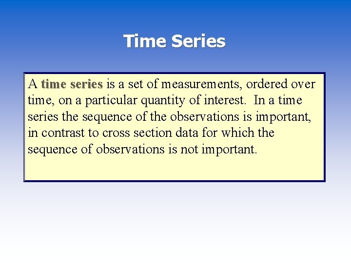
Time Series A time series is a set of measurements, ordered over time, on a particular quantity of interest. In a time series the sequence of the observations is important, in contrast to cross section data for which the sequence of observations is not important.

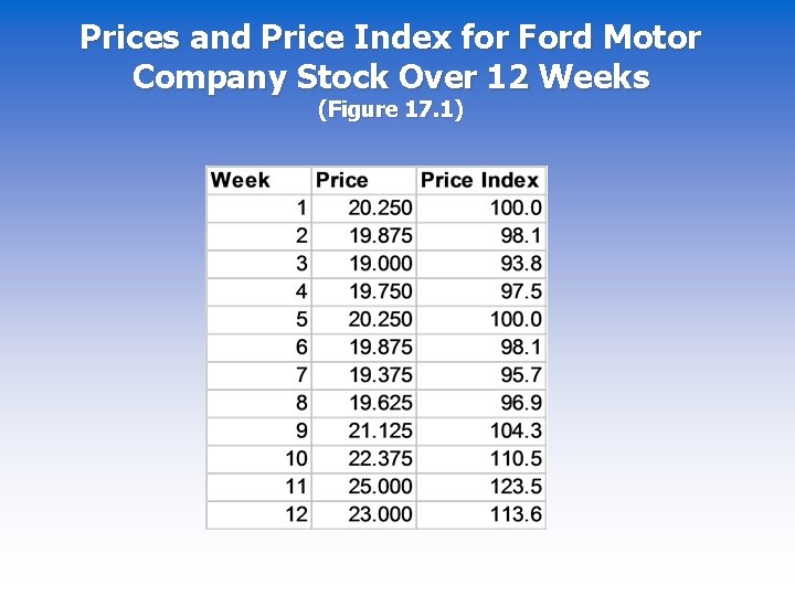
Prices and Price Index for Ford Motor Company Stock Over 12 Weeks (Figure 17. 1)

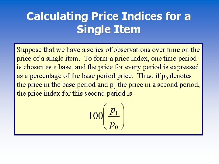
Calculating Price Indices for a Single Item Suppose that we have a series of observations over time on the price of a single item. To form a price index, one time period is chosen as a base, and the price for every period is expressed as a percentage of the base period price. Thus, if p 0 denotes the price in the base period and p 1 the price in a second period, the price index for this second period is

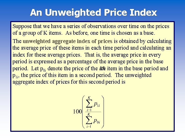
An Unweighted Price Index Suppose that we have a series of observations over time on the prices of a group of K items. As before, one time is chosen as a base. The unweighted aggregate index of prices is obtained by calculating the average price of these items in each time period and calculating an index for these average prices. That is, the average price in every period is expressed as a percentage of the average price in the base period. Let p 0 i denote the price of the ith item in the base period and p 1 i, the price of this item in a second period. The unweighted aggregate index of prices for this second period is

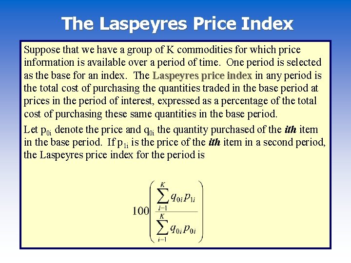
The Laspeyres Price Index Suppose that we have a group of K commodities for which price information is available over a period of time. One period is selected as the base for an index. The Laspeyres price index in any period is the total cost of purchasing the quantities traded in the base period at prices in the period of interest, expressed as a percentage of the total cost of purchasing these same quantities in the base period. Let p 0 i denote the price and q 0 i the quantity purchased of the ith item in the base period. If p 1 i is the price of the ith item in a second period, the Laspeyres price index for the period is

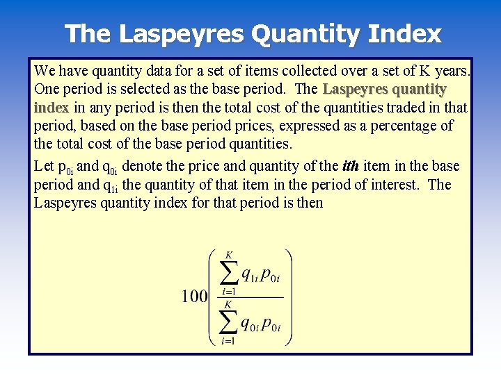
The Laspeyres Quantity Index We have quantity data for a set of items collected over a set of K years. One period is selected as the base period. The Laspeyres quantity index in any period is then the total cost of the quantities traded in that period, based on the base period prices, expressed as a percentage of the total cost of the base period quantities. Let p 0 i and q 0 i denote the price and quantity of the ith item in the base period and q 1 i the quantity of that item in the period of interest. The Laspeyres quantity index for that period is then

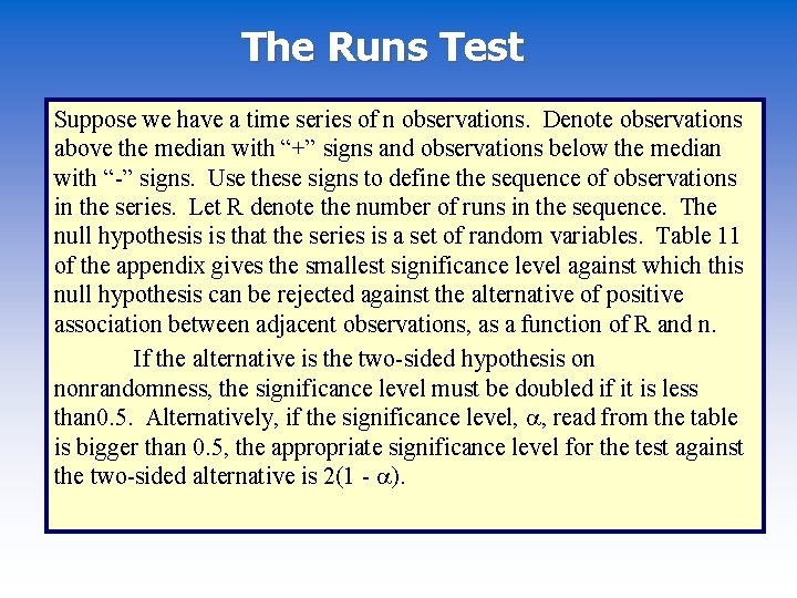
The Runs Test Suppose we have a time series of n observations. Denote observations above the median with “+” signs and observations below the median with “-” signs. Use these signs to define the sequence of observations in the series. Let R denote the number of runs in the sequence. The null hypothesis is that the series is a set of random variables. Table 11 of the appendix gives the smallest significance level against which this null hypothesis can be rejected against the alternative of positive association between adjacent observations, as a function of R and n. If the alternative is the two-sided hypothesis on nonrandomness, the significance level must be doubled if it is less than 0. 5. Alternatively, if the significance level, , read from the table is bigger than 0. 5, the appropriate significance level for the test against the two-sided alternative is 2(1 - ).

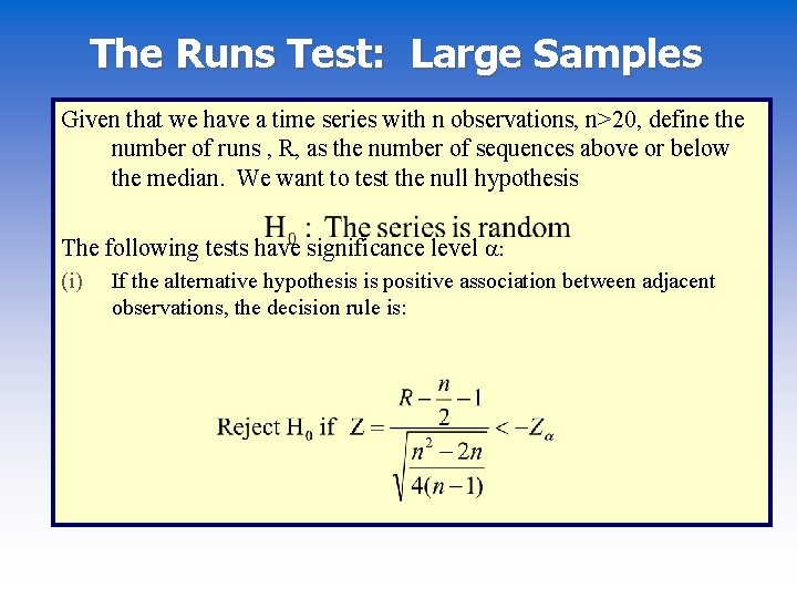
The Runs Test: Large Samples Given that we have a time series with n observations, n>20, define the number of runs , R, as the number of sequences above or below the median. We want to test the null hypothesis The following tests have significance level : (i) If the alternative hypothesis is positive association between adjacent observations, the decision rule is:

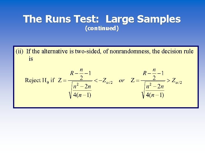
The Runs Test: Large Samples (continued) (ii) If the alternative is two-sided, of nonrandomness, the decision rule is

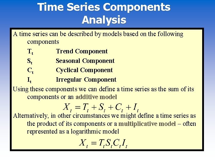
Time Series Components Analysis A time series can be described by models based on the following components Tt Trend Component St Seasonal Component Ct Cyclical Component It Irregular Component Using these components we can define a time series as the sum of its components or an additive model Alternatively, in other circumstances we might define a time series as the product of its components or a multiplicative model – often represented as a logarithmic model

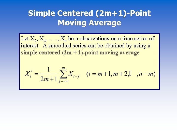
Simple Centered (2 m+1)-Point Moving Average Let X 1, X 2, . . . , Xn be n observations on a time series of interest. A smoothed series can be obtained by using a simple centered (2 m + 1)-point moving average

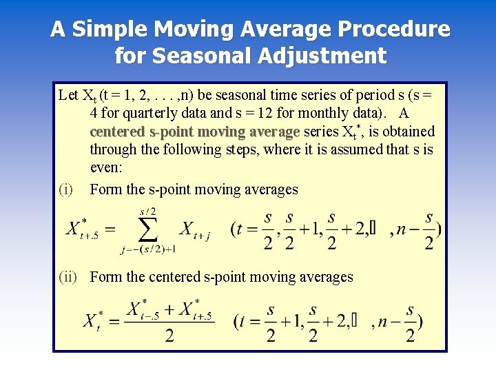
A Simple Moving Average Procedure for Seasonal Adjustment Let Xt (t = 1, 2, . . . , n) be seasonal time series of period s (s = 4 for quarterly data and s = 12 for monthly data). A centered s-point moving average series Xt*, is obtained through the following steps, where it is assumed that s is even: (i) Form the s-point moving averages (ii) Form the centered s-point moving averages

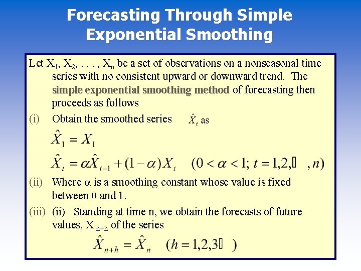
Forecasting Through Simple Exponential Smoothing Let X 1, X 2, . . . , Xn be a set of observations on a nonseasonal time series with no consistent upward or downward trend. The simple exponential smoothing method of forecasting then proceeds as follows (i) Obtain the smoothed series (ii) Where is a smoothing constant whose value is fixed between 0 and 1. (iii) (ii) Standing at time n, we obtain the forecasts of future values, X n+h of the series

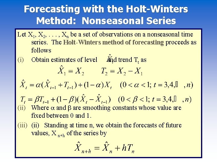
Forecasting with the Holt-Winters Method: Nonseasonal Series Let X 1, X 2, . . . , Xn be a set of observations on a nonseasonal time series. The Holt-Winters method of forecasting proceeds as follows (i) Obtain estimates of level and trend Tt as (ii) Where and are smoothing constants whose value are fixed between 0 and 1. (iii) (ii) Standing at time n, we obtain the forecasts of future values, X n+h of the series by

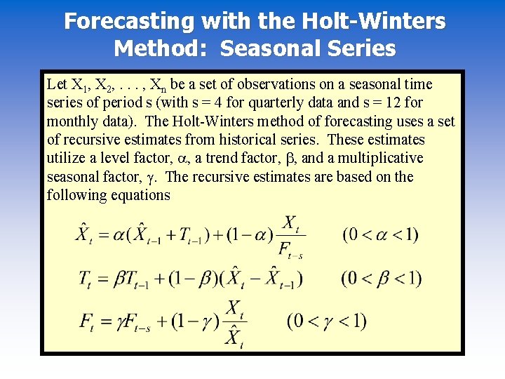
Forecasting with the Holt-Winters Method: Seasonal Series Let X 1, X 2, . . . , Xn be a set of observations on a seasonal time series of period s (with s = 4 for quarterly data and s = 12 for monthly data). The Holt-Winters method of forecasting uses a set of recursive estimates from historical series. These estimates utilize a level factor, , a trend factor, , and a multiplicative seasonal factor, . The recursive estimates are based on the following equations

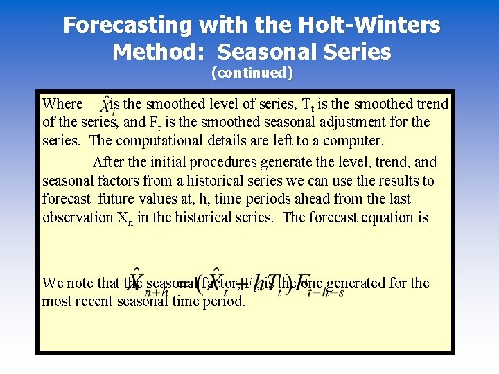
Forecasting with the Holt-Winters Method: Seasonal Series (continued) Where is the smoothed level of series, Tt is the smoothed trend of the series, and Ft is the smoothed seasonal adjustment for the series. The computational details are left to a computer. After the initial procedures generate the level, trend, and seasonal factors from a historical series we can use the results to forecast future values at, h, time periods ahead from the last observation Xn in the historical series. The forecast equation is We note that the seasonal factor, Ft, is the one generated for the most recent seasonal time period.

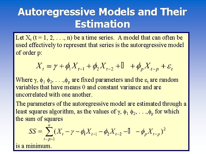
Autoregressive Models and Their Estimation Let Xt (t = 1, 2, . . . , n) be a time series. A model that can often be used effectively to represent that series is the autoregressive model of order p: Where , 1 2, . . . , p are fixed parameters and the t are random variables that have means 0 and constant variance and are uncorrelated with one another. The parameters of the autoregressive model are estimated through a least squares algorithm, as the values of , 1 2, . . . , p for which the sum of squares is a minimum.

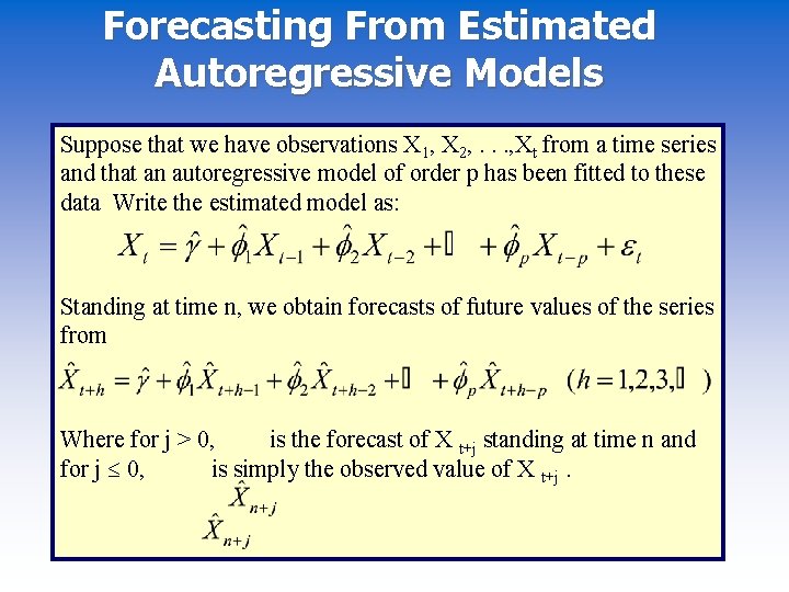
Forecasting From Estimated Autoregressive Models Suppose that we have observations X 1, X 2, . . . , Xt from a time series and that an autoregressive model of order p has been fitted to these data Write the estimated model as: Standing at time n, we obtain forecasts of future values of the series from Where for j > 0, is the forecast of X t+j standing at time n and for j 0, is simply the observed value of X t+j.

Key Words 4 ARIMA Models 4 Autoregressive Models and Their Estimation 4 Calculating Price Indices for a Single Item 4 Change in Base Period 4 Forecasting with the Holt. Winters Method: Nonseasonal Series 4 Forecasting with the Holt. Winters Method: Seasonal Series 4 Forecasting From Estimated Autoregressive Models 4 Forecasting Through Simple Exponential Smoothing 4 Index Numbers 4 Laspeyres Price Index 4 Runs Test: Large Samples 4 Simple Centered (2 m+1)Point Moving Averages 4 Simple Exponential Smoothing 4 Simple Moving Average Procedure for Seasonal Adjustment

Key Words (continued) 4 Spliced Price Index 4 Time Series Components Analysis 4 Unweighted Price Index 4 Weighted Aggregate Quantity Index 4 Weighted Price Index