Chapter 17 Output and the Exchange Rate in

Chapter 17 Output and the Exchange Rate in the Short Run Copyright © 2012 Pearson Education. All rights reserved.

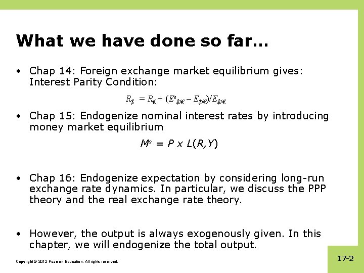
What we have done so far… • Chap 14: Foreign exchange market equilibrium gives: Interest Parity Condition: R$ = R€ + (Ee$/€ – E$/€)/E$/€ • Chap 15: Endogenize nominal interest rates by introducing money market equilibrium Ms = P x L(R, Y) • Chap 16: Endogenize expectation by considering long-run exchange rate dynamics. In particular, we discuss the PPP theory and the real exchange rate theory. • However, the output is always exogenously given. In this chapter, we will endogenize the total output. Copyright © 2012 Pearson Education. All rights reserved. 17 -2

Preview • Determinants of aggregate demand in the short run • A short-run model of output markets • A short-run model of asset markets • A short-run model for both output markets and asset markets • Effects of temporary and permanent changes in monetary and fiscal policies • Adjustment of the current account over time Copyright © 2012 Pearson Education. All rights reserved. 17 -3

Introduction • Long-run models are useful when all prices of inputs and outputs have time to adjust. • In the short run, some prices of inputs and outputs may not have time to adjust, due to labor contracts, costs of adjustment, or imperfect information about willingness of customers to pay at different prices. Thus, demand determines the equilibrium output given sticky price. • This chapter builds on the short-run and long-run models of exchange rates to explain how output is related to exchange rates in the short run. – It shows how macroeconomic policies can affect production, employment, and the current account. Copyright © 2012 Pearson Education. All rights reserved. 17 -4

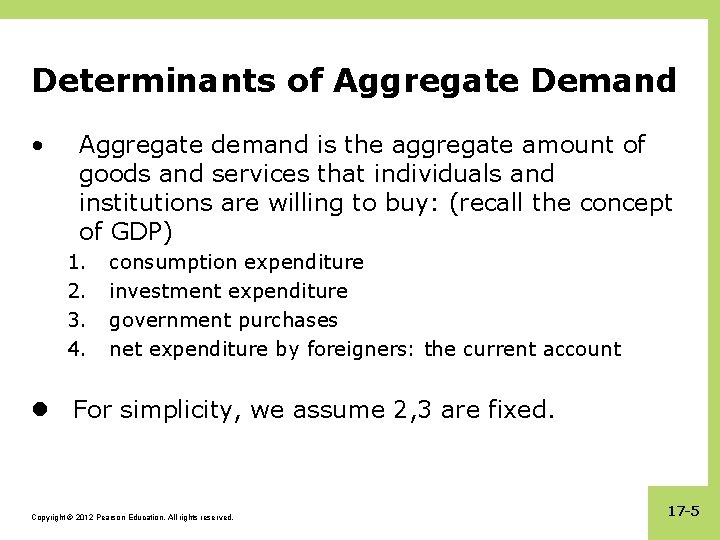
Determinants of Aggregate Demand • Aggregate demand is the aggregate amount of goods and services that individuals and institutions are willing to buy: (recall the concept of GDP) 1. 2. 3. 4. consumption expenditure investment expenditure government purchases net expenditure by foreigners: the current account l For simplicity, we assume 2, 3 are fixed. Copyright © 2012 Pearson Education. All rights reserved. 17 -5

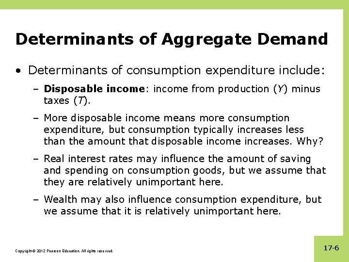
Determinants of Aggregate Demand • Determinants of consumption expenditure include: – Disposable income: income from production (Y) minus taxes (T). – More disposable income means more consumption expenditure, but consumption typically increases less than the amount that disposable income increases. Why? – Real interest rates may influence the amount of saving and spending on consumption goods, but we assume that they are relatively unimportant here. – Wealth may also influence consumption expenditure, but we assume that it is relatively unimportant here. Copyright © 2012 Pearson Education. All rights reserved. 17 -6

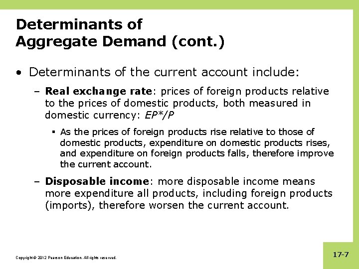
Determinants of Aggregate Demand (cont. ) • Determinants of the current account include: – Real exchange rate: prices of foreign products relative to the prices of domestic products, both measured in domestic currency: EP*/P § As the prices of foreign products rise relative to those of domestic products, expenditure on domestic products rises, and expenditure on foreign products falls, therefore improve the current account. – Disposable income: more disposable income means more expenditure all products, including foreign products (imports), therefore worsen the current account. Copyright © 2012 Pearson Education. All rights reserved. 17 -7

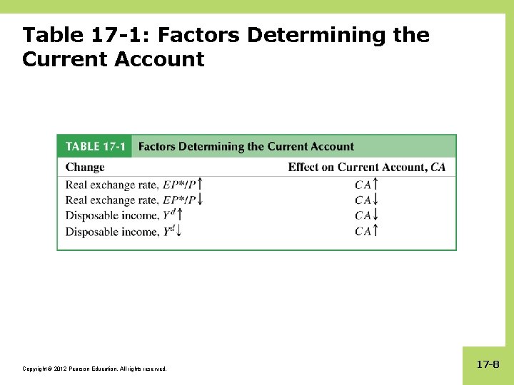
Table 17 -1: Factors Determining the Current Account Copyright © 2012 Pearson Education. All rights reserved. 17 -8

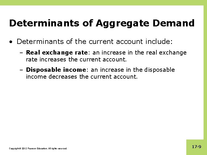
Determinants of Aggregate Demand • Determinants of the current account include: – Real exchange rate: an increase in the real exchange rate increases the current account. – Disposable income: an increase in the disposable income decreases the current account. Copyright © 2012 Pearson Education. All rights reserved. 17 -9

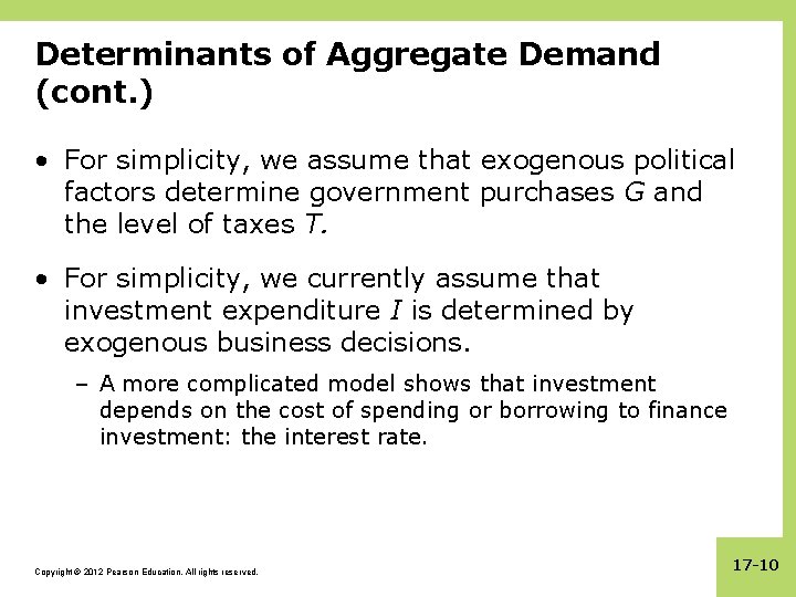
Determinants of Aggregate Demand (cont. ) • For simplicity, we assume that exogenous political factors determine government purchases G and the level of taxes T. • For simplicity, we currently assume that investment expenditure I is determined by exogenous business decisions. – A more complicated model shows that investment depends on the cost of spending or borrowing to finance investment: the interest rate. Copyright © 2012 Pearson Education. All rights reserved. 17 -10

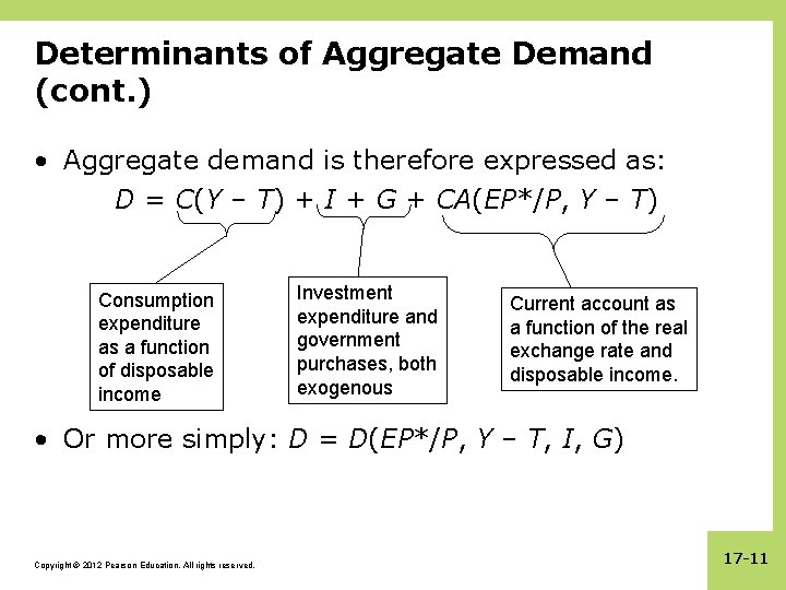
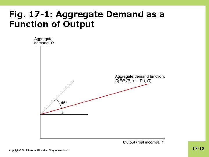
Determinants of Aggregate Demand (cont. ) • Aggregate demand is therefore expressed as: D = C(Y – T) + I + G + CA(EP*/P, Y – T) Consumption expenditure as a function of disposable income Investment expenditure and government purchases, both exogenous Current account as a function of the real exchange rate and disposable income. • Or more simply: D = D(EP*/P, Y – T, I, G) Copyright © 2012 Pearson Education. All rights reserved. 17 -11

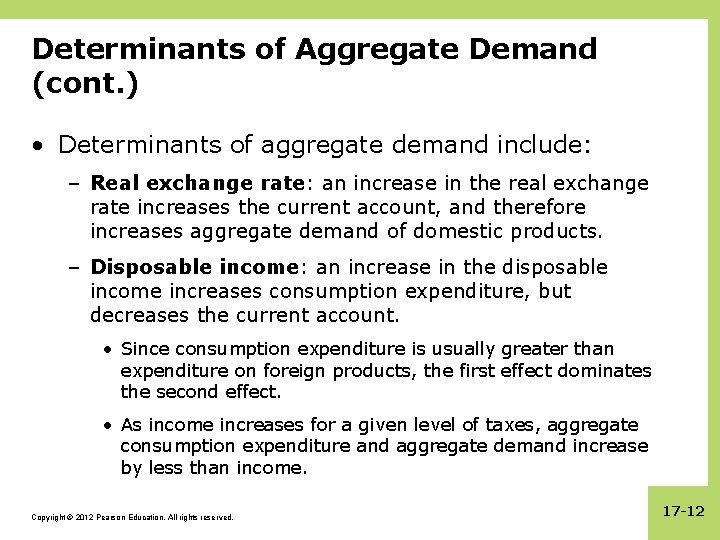
Determinants of Aggregate Demand (cont. ) • Determinants of aggregate demand include: – Real exchange rate: an increase in the real exchange rate increases the current account, and therefore increases aggregate demand of domestic products. – Disposable income: an increase in the disposable income increases consumption expenditure, but decreases the current account. • Since consumption expenditure is usually greater than expenditure on foreign products, the first effect dominates the second effect. • As income increases for a given level of taxes, aggregate consumption expenditure and aggregate demand increase by less than income. Copyright © 2012 Pearson Education. All rights reserved. 17 -12

Fig. 17 -1: Aggregate Demand as a Function of Output Copyright © 2012 Pearson Education. All rights reserved. 17 -13

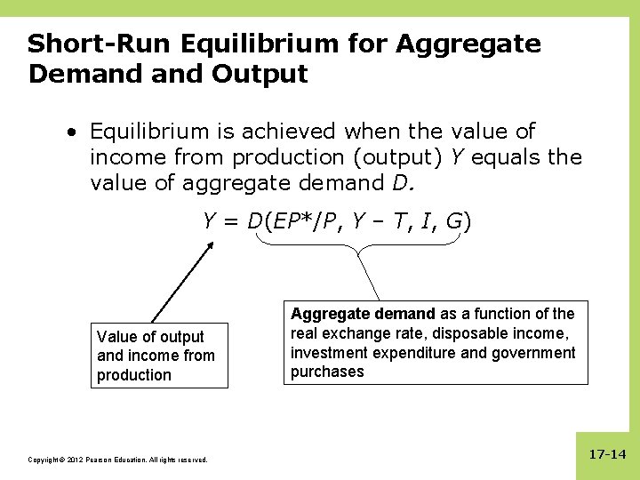
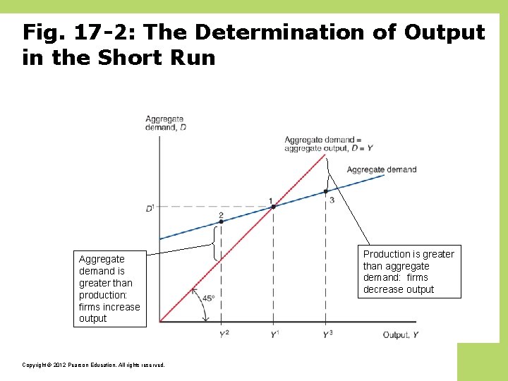
Short-Run Equilibrium for Aggregate Demand Output • Equilibrium is achieved when the value of income from production (output) Y equals the value of aggregate demand D. Y = D(EP*/P, Y – T, I, G) Value of output and income from production Copyright © 2012 Pearson Education. All rights reserved. Aggregate demand as a function of the real exchange rate, disposable income, investment expenditure and government purchases 17 -14

Fig. 17 -2: The Determination of Output in the Short Run Aggregate demand is greater than production: firms increase output Copyright © 2012 Pearson Education. All rights reserved. Production is greater than aggregate demand: firms decrease output

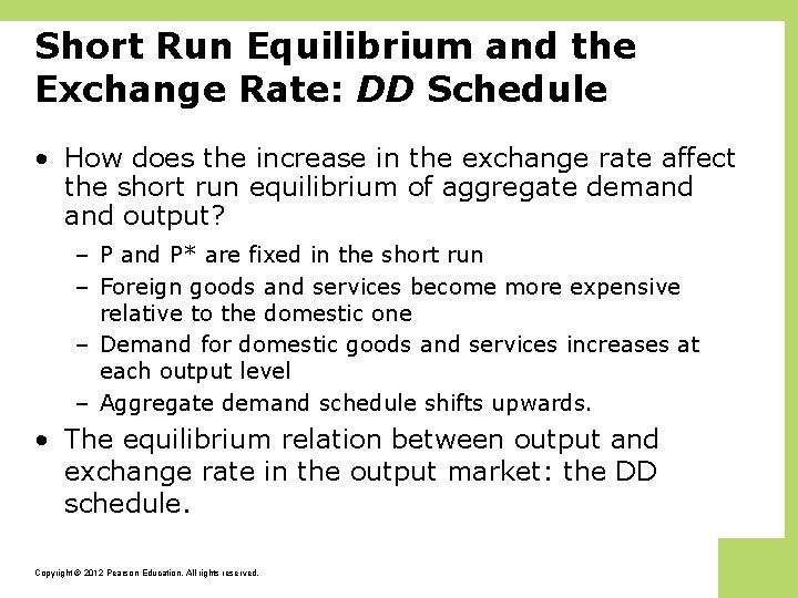
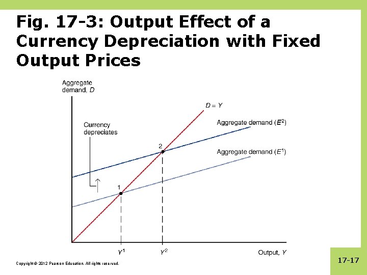
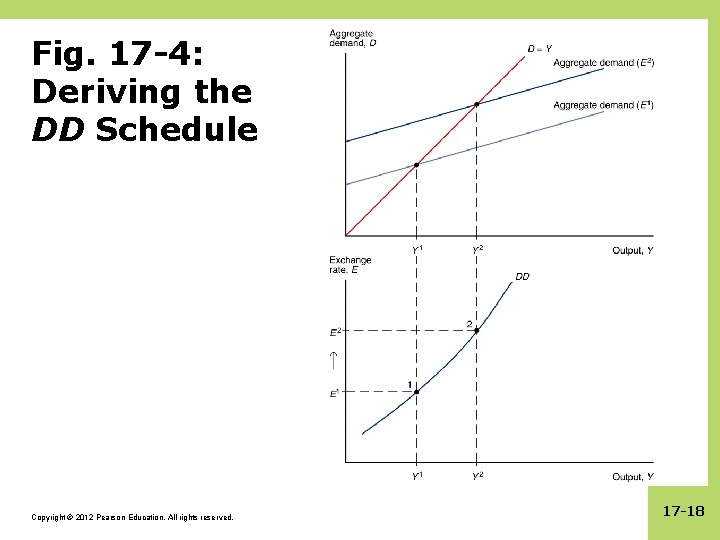
Short Run Equilibrium and the Exchange Rate: DD Schedule • How does the increase in the exchange rate affect the short run equilibrium of aggregate demand output? – P and P* are fixed in the short run – Foreign goods and services become more expensive relative to the domestic one – Demand for domestic goods and services increases at each output level – Aggregate demand schedule shifts upwards. • The equilibrium relation between output and exchange rate in the output market: the DD schedule. Copyright © 2012 Pearson Education. All rights reserved.

Fig. 17 -3: Output Effect of a Currency Depreciation with Fixed Output Prices Copyright © 2012 Pearson Education. All rights reserved. 17 -17

Fig. 17 -4: Deriving the DD Schedule Copyright © 2012 Pearson Education. All rights reserved. 17 -18

Short-Run Equilibrium and the Exchange Rate: DD Schedule (cont. ) DD schedule • shows combinations of output and the exchange rate at which the output market is in short-run equilibrium (such that aggregate demand = aggregate output). • slopes upward because a rise in the exchange rate causes aggregate demand aggregate output to rise. Copyright © 2012 Pearson Education. All rights reserved. 17 -19

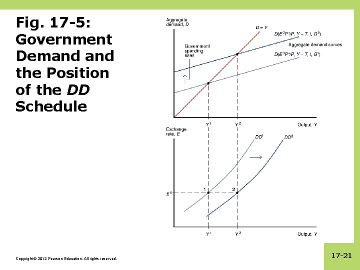
Shifting the DD Curve • Changes in the exchange rate cause movements along a DD curve. Other changes cause it to shift: 1. Changes in G: more government purchases cause higher aggregate demand output in equilibrium. Output increases for every exchange rate: the DD curve shifts right. Copyright © 2012 Pearson Education. All rights reserved. 17 -20

Fig. 17 -5: Government Demand the Position of the DD Schedule Copyright © 2012 Pearson Education. All rights reserved. 17 -21

Shifting the DD Curve (cont. ) 2. Changes in T: lower taxes generally increase consumption expenditure, increasing aggregate demand output in equilibrium for every exchange rate: the DD curve shifts right. 3. Changes in I: higher investment expenditure is represented by shifting the DD curve right. 4. Changes in P relative to P*: lower domestic prices relative to foreign prices are represented by shifting the DD curve right. Copyright © 2012 Pearson Education. All rights reserved. 17 -22

Shifting the DD Curve (cont. ) 5. Changes in C: willingness to consume more and save less is represented by shifting the DD curve right. 6. Changes in demand of domestic goods relative to foreign goods: willingness to consume more domestic goods relative to foreign goods is represented by shifting the DD curve right. Copyright © 2012 Pearson Education. All rights reserved. 17 -23

Shifting the DD Curve (cont. ) • Any disturbance domestic output the right. • Any disturbance domestic output the left. Copyright © 2012 Pearson Education. All rights reserved. that increase AD for shifts the DD schedule to that lowers AD for shifts the DD schedule to

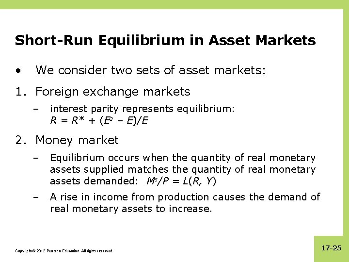
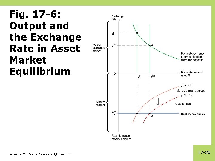
Short-Run Equilibrium in Asset Markets • We consider two sets of asset markets: 1. Foreign exchange markets – interest parity represents equilibrium: R = R* + (Ee – E)/E 2. Money market – Equilibrium occurs when the quantity of real monetary assets supplied matches the quantity of real monetary assets demanded: Ms/P = L(R, Y) – A rise in income from production causes the demand of real monetary assets to increase. Copyright © 2012 Pearson Education. All rights reserved. 17 -25

Fig. 17 -6: Output and the Exchange Rate in Asset Market Equilibrium Copyright © 2012 Pearson Education. All rights reserved. 17 -26

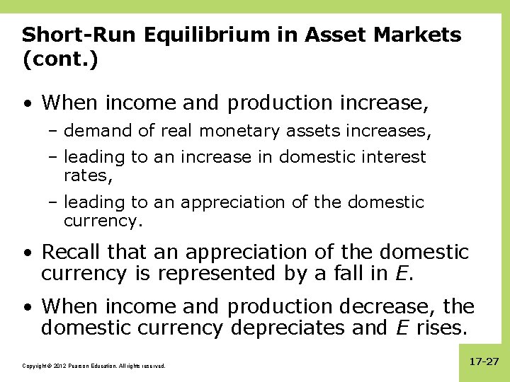
Short-Run Equilibrium in Asset Markets (cont. ) • When income and production increase, – demand of real monetary assets increases, – leading to an increase in domestic interest rates, – leading to an appreciation of the domestic currency. • Recall that an appreciation of the domestic currency is represented by a fall in E. • When income and production decrease, the domestic currency depreciates and E rises. Copyright © 2012 Pearson Education. All rights reserved. 17 -27

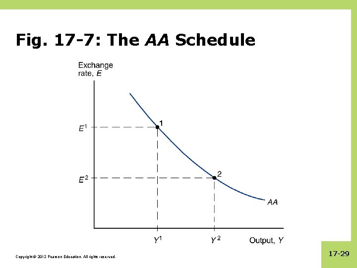
Short-Run Equilibrium in Asset Markets: AA Curve • The inverse relationship between output and exchange rates needed to keep the foreign exchange markets and the money market in equilibrium is summarized as the AA curve. Copyright © 2012 Pearson Education. All rights reserved. 17 -28

Fig. 17 -7: The AA Schedule Copyright © 2012 Pearson Education. All rights reserved. 17 -29

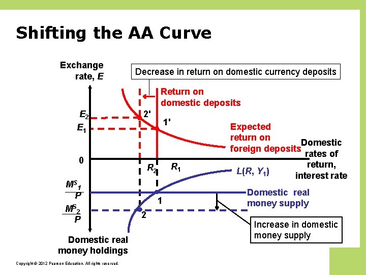
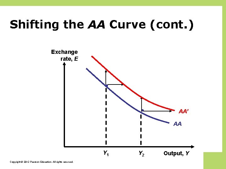
Shifting the AA Curve 1. Changes in Ms: an increase in the money supply reduces interest rates in the short run, causing the domestic currency to depreciate (a rise in E) for every Y: the AA curve shifts up (right). Copyright © 2012 Pearson Education. All rights reserved. 17 -30

Shifting the AA Curve Exchange rate, E Decrease in return on domestic currency deposits Return on domestic deposits E 2 E 1 2' 0 MS 1 P MS 2 P Domestic real money holdings Copyright © 2012 Pearson Education. All rights reserved. 1' R 1 R 2 1 2 Expected return on Domestic foreign deposits rates of return, L(R, Y 1) interest rate Domestic real money supply Increase in domestic money supply

Shifting the AA Curve (cont. ) Exchange rate, E AA’ AA Y 1 Copyright © 2012 Pearson Education. All rights reserved. Y 2 Output, Y

Shifting the AA Curve (cont. ) 2. Changes in P: An increase in the level of average domestic prices decreases the supply of real monetary assets, increasing interest rates, causing the domestic currency to appreciate (a fall in E): the AA curve shifts down (left). 3. Changes in the demand of real monetary assets: if domestic residents are willing to hold a lower amount of real money assets and more nonmonetary assets, interest rates on nonmonetary assets would fall, leading to a depreciation of the domestic currency (a rise in E): the AA curve shifts up (right). Copyright © 2012 Pearson Education. All rights reserved. 17 -33

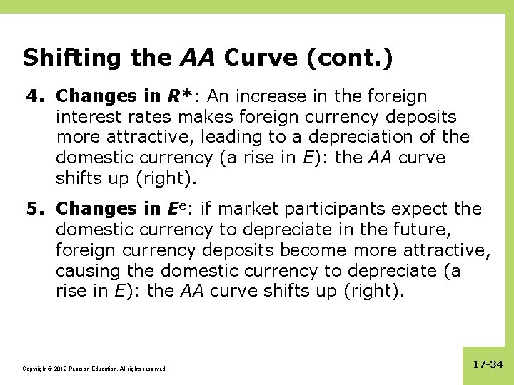
Shifting the AA Curve (cont. ) 4. Changes in R*: An increase in the foreign interest rates makes foreign currency deposits more attractive, leading to a depreciation of the domestic currency (a rise in E): the AA curve shifts up (right). 5. Changes in Ee: if market participants expect the domestic currency to depreciate in the future, foreign currency deposits become more attractive, causing the domestic currency to depreciate (a rise in E): the AA curve shifts up (right). Copyright © 2012 Pearson Education. All rights reserved. 17 -34

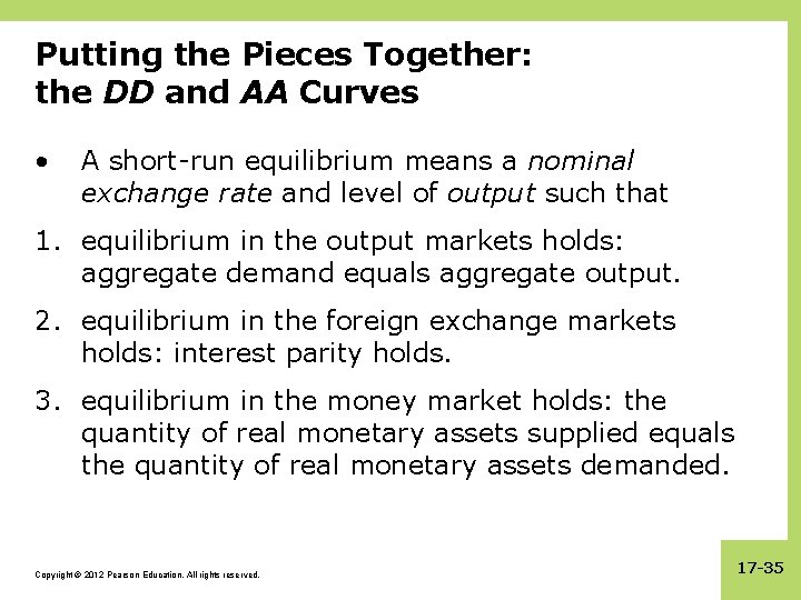
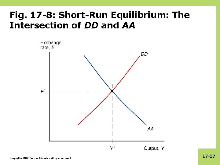
Putting the Pieces Together: the DD and AA Curves • A short-run equilibrium means a nominal exchange rate and level of output such that 1. equilibrium in the output markets holds: aggregate demand equals aggregate output. 2. equilibrium in the foreign exchange markets holds: interest parity holds. 3. equilibrium in the money market holds: the quantity of real monetary assets supplied equals the quantity of real monetary assets demanded. Copyright © 2012 Pearson Education. All rights reserved. 17 -35

Putting the Pieces Together: the DD and AA Curves (cont. ) • A short-run equilibrium occurs at the intersection of the DD and AA curves: – output markets are in equilibrium on the DD curve – asset markets are in equilibrium on the AA curve Copyright © 2012 Pearson Education. All rights reserved. 17 -36

Fig. 17 -8: Short-Run Equilibrium: The Intersection of DD and AA Copyright © 2012 Pearson Education. All rights reserved. 17 -37

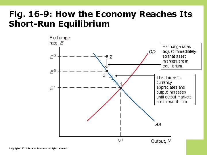
Fig. 16 -9: How the Economy Reaches Its Short-Run Equilibrium Exchange rates adjust immediately so that asset markets are in equilibrium. The domestic currency appreciates and output increases until output markets are in equilibrium. Copyright © 2012 Pearson Education. All rights reserved.

Temporary Changes in Monetary and Fiscal Policy • Monetary policy: policy in which the central bank influences the supply of monetary assets. – Monetary policy is assumed to affect asset markets first. • Fiscal policy: policy in which governments (fiscal authorities) influence the amount of government purchases and taxes. – Fiscal policy is assumed to affect aggregate demand output first. • Temporary policy changes are expected to be reversed in the near future and thus do not affect expectations about exchange rates in the long run. Copyright © 2012 Pearson Education. All rights reserved. 17 -39

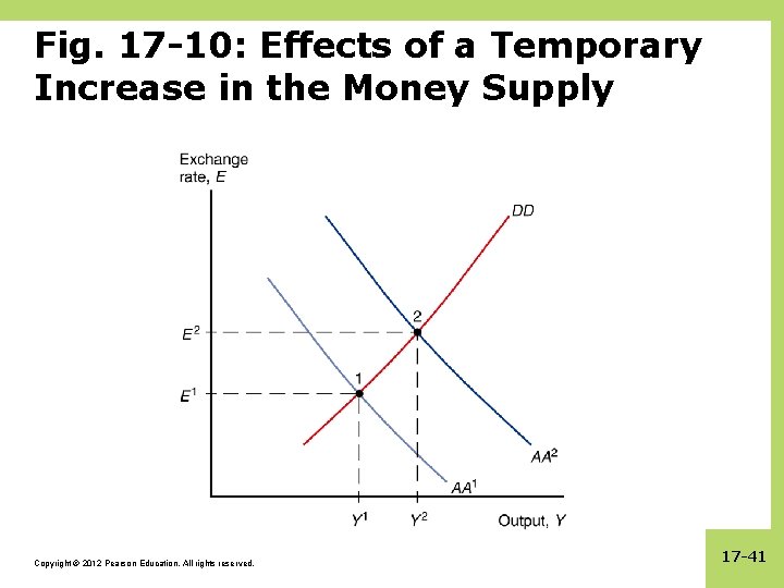
Temporary Changes in Monetary Policy • An increase in the quantity of monetary assets supplied lowers interest rates in the short run, causing the domestic currency to depreciate (E rises). – The AA shifts up (right). – Domestic products relative to foreign products are cheaper, so that aggregate demand output increase until a new short-run equilibrium is achieved. Copyright © 2012 Pearson Education. All rights reserved. 17 -40

Fig. 17 -10: Effects of a Temporary Increase in the Money Supply Copyright © 2012 Pearson Education. All rights reserved. 17 -41

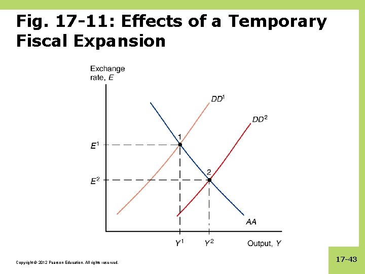
Temporary Changes in Fiscal Policy • An increase in government purchases or a decrease in taxes increases aggregate demand output in the short run. – The DD curve shifts right. – Higher output increases the demand for real monetary assets, • thereby increasing interest rates, • causing the domestic currency to appreciate (E falls). Copyright © 2012 Pearson Education. All rights reserved. 17 -42

Fig. 17 -11: Effects of a Temporary Fiscal Expansion Copyright © 2012 Pearson Education. All rights reserved. 17 -43

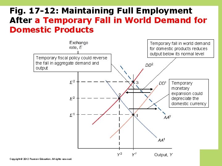
Policies to Maintain Full Employment • Resources used in the production process can either be overemployed or underemployed. • When resources are used effectively and sustainably, economists say that production is at its potential or natural level. – When resources are not used effectively, resources are underemployed: high unemployment, few hours worked, idle equipment, lower than normal production of goods and services. – When resources are not used sustainably, labor is overemployed: low unemployment, many overtime hours, overutilized equipment, higher than normal production of goods and services. Copyright © 2012 Pearson Education. All rights reserved. 17 -44

Fig. 17 -12: Maintaining Full Employment After a Temporary Fall in World Demand for Domestic Products Temporary fiscal policy could reverse the fall in aggregate demand output Temporary fall in world demand for domestic products reduces output below its normal level Temporary monetary expansion could depreciate the domestic currency Copyright © 2012 Pearson Education. All rights reserved.

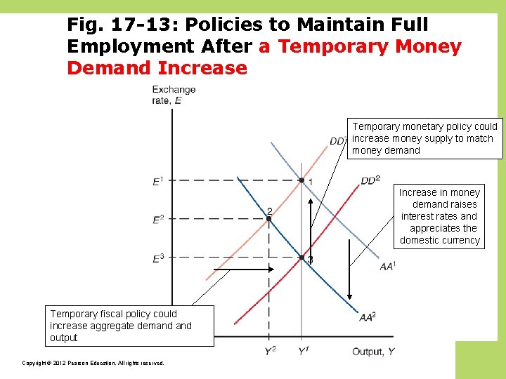
Fig. 17 -13: Policies to Maintain Full Employment After a Temporary Money Demand Increase Temporary monetary policy could increase money supply to match money demand Increase in money demand raises interest rates and appreciates the domestic currency Temporary fiscal policy could increase aggregate demand output Copyright © 2012 Pearson Education. All rights reserved.

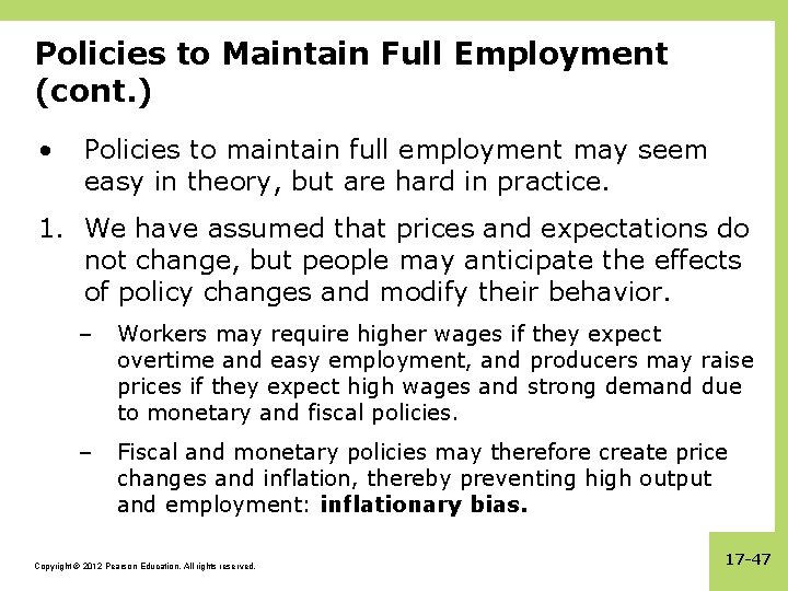
Policies to Maintain Full Employment (cont. ) • Policies to maintain full employment may seem easy in theory, but are hard in practice. 1. We have assumed that prices and expectations do not change, but people may anticipate the effects of policy changes and modify their behavior. – Workers may require higher wages if they expect overtime and easy employment, and producers may raise prices if they expect high wages and strong demand due to monetary and fiscal policies. – Fiscal and monetary policies may therefore create price changes and inflation, thereby preventing high output and employment: inflationary bias. Copyright © 2012 Pearson Education. All rights reserved. 17 -47

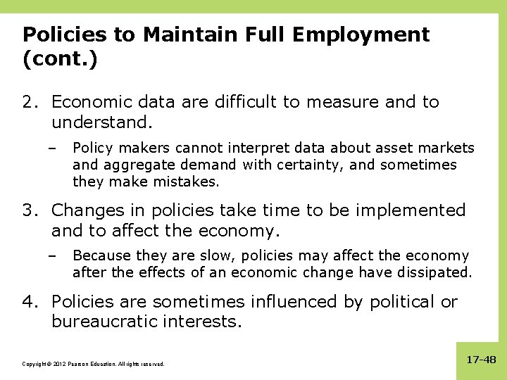
Policies to Maintain Full Employment (cont. ) 2. Economic data are difficult to measure and to understand. – Policy makers cannot interpret data about asset markets and aggregate demand with certainty, and sometimes they make mistakes. 3. Changes in policies take time to be implemented and to affect the economy. – Because they are slow, policies may affect the economy after the effects of an economic change have dissipated. 4. Policies are sometimes influenced by political or bureaucratic interests. Copyright © 2012 Pearson Education. All rights reserved. 17 -48

Permanent Changes in Monetary and Fiscal Policy • “Permanent” policy changes are those that are assumed to modify people’s expectations about exchange rates in the long run. Copyright © 2012 Pearson Education. All rights reserved. 17 -49

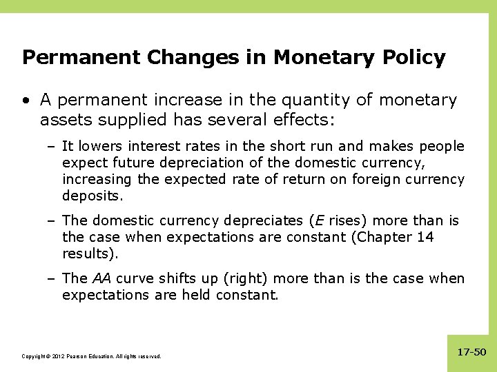
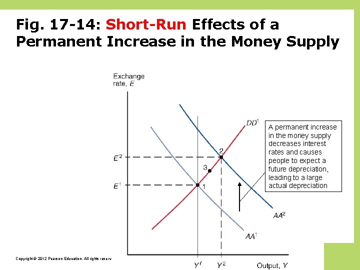
Permanent Changes in Monetary Policy • A permanent increase in the quantity of monetary assets supplied has several effects: – It lowers interest rates in the short run and makes people expect future depreciation of the domestic currency, increasing the expected rate of return on foreign currency deposits. – The domestic currency depreciates (E rises) more than is the case when expectations are constant (Chapter 14 results). – The AA curve shifts up (right) more than is the case when expectations are held constant. Copyright © 2012 Pearson Education. All rights reserved. 17 -50

Fig. 17 -14: Short-Run Effects of a Permanent Increase in the Money Supply A permanent increase in the money supply decreases interest rates and causes people to expect a future depreciation, leading to a large actual depreciation Copyright © 2012 Pearson Education. All rights reserved.

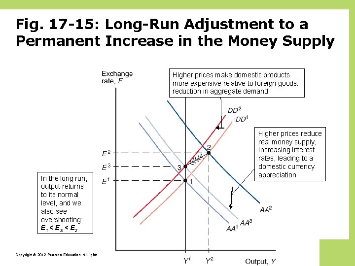
Effects of Permanent Changes in Monetary Policy in the Long Run • With employment and hours above their normal levels, there is a tendency for wages to rise over time. • With strong demand for goods and services and with increasing wages, producers have an incentive to raise prices over time. • Both higher wages and higher output prices are reflected in a higher level of average prices. • What are the effects of rising prices? Copyright © 2012 Pearson Education. All rights reserved. 17 -52

Fig. 17 -15: Long-Run Adjustment to a Permanent Increase in the Money Supply Higher prices make domestic products more expensive relative to foreign goods: reduction in aggregate demand In the long run, output returns to its normal level, and we also see overshooting: E 1 < E 3 < E 2 Copyright © 2012 Pearson Education. All rights reserved. Higher prices reduce real money supply, Increasing interest rates, leading to a domestic currency appreciation

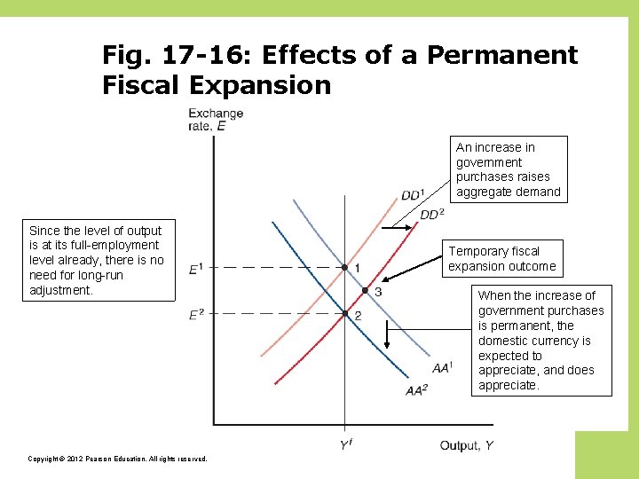
Effects of Permanent Changes in Fiscal Policy • A permanent increase in government purchases or reduction in taxes – increases aggregate demand – makes people expect the domestic currency to appreciate in the long run due to increased aggregate demand, thereby reducing the expected rate of return on foreign currency deposits and making the domestic currency appreciate. • The first effect increases aggregate demand of domestic products, the second effect decreases aggregate demand of domestic products (by making them more expensive). Copyright © 2012 Pearson Education. All rights reserved. 17 -54

Effects of Permanent Changes in Fiscal Policy (cont. ) • If the change in fiscal policy is expected to be permanent, the first and second effects exactly offset each other, so that output remains at its potential or natural (or long run) level. • We say that an increase in government purchases completely crowds out net exports, due to the effect of the appreciated domestic currency. Copyright © 2012 Pearson Education. All rights reserved. 17 -55

Fig. 17 -16: Effects of a Permanent Fiscal Expansion An increase in government purchases raises aggregate demand Since the level of output is at its full-employment level already, there is no need for long-run adjustment. Copyright © 2012 Pearson Education. All rights reserved. Temporary fiscal expansion outcome When the increase of government purchases is permanent, the domestic currency is expected to appreciate, and does appreciate.

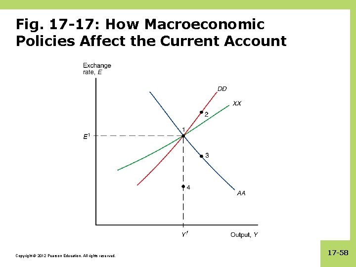
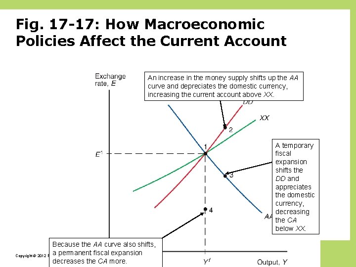
Macroeconomic Policies and the Current Account • To determine the effect of monetary and fiscal policies on the current account, – derive the XX curve to represent the combinations of output and exchange rates at which the current account is at its desired level. • As income from production increases, imports increase and the current account decreases when other factors remain constant. • To keep the current account at its desired level, the domestic currency must depreciate as income from production increases: the XX curve should slope upward. Copyright © 2012 Pearson Education. All rights reserved. 17 -57

Fig. 17 -17: How Macroeconomic Policies Affect the Current Account Copyright © 2012 Pearson Education. All rights reserved. 17 -58

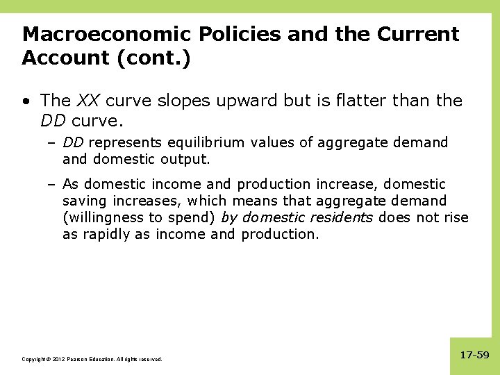
Macroeconomic Policies and the Current Account (cont. ) • The XX curve slopes upward but is flatter than the DD curve. – DD represents equilibrium values of aggregate demand domestic output. – As domestic income and production increase, domestic saving increases, which means that aggregate demand (willingness to spend) by domestic residents does not rise as rapidly as income and production. Copyright © 2012 Pearson Education. All rights reserved. 17 -59

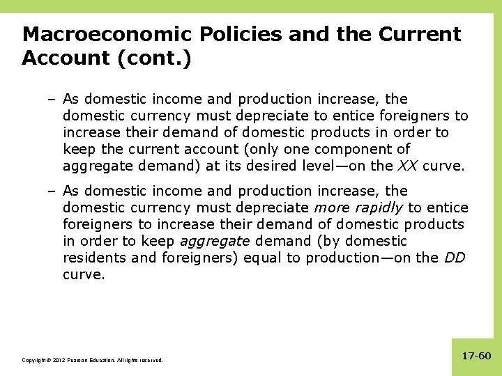
Macroeconomic Policies and the Current Account (cont. ) – As domestic income and production increase, the domestic currency must depreciate to entice foreigners to increase their demand of domestic products in order to keep the current account (only one component of aggregate demand) at its desired level—on the XX curve. – As domestic income and production increase, the domestic currency must depreciate more rapidly to entice foreigners to increase their demand of domestic products in order to keep aggregate demand (by domestic residents and foreigners) equal to production—on the DD curve. Copyright © 2012 Pearson Education. All rights reserved. 17 -60

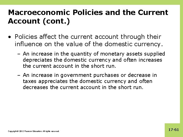
Macroeconomic Policies and the Current Account (cont. ) • Policies affect the current account through their influence on the value of the domestic currency. – An increase in the quantity of monetary assets supplied depreciates the domestic currency and often increases the current account in the short run. – An increase in government purchases or decrease in taxes appreciates the domestic currency and often decreases the current account in the short run. Copyright © 2012 Pearson Education. All rights reserved. 17 -61

Fig. 17 -17: How Macroeconomic Policies Affect the Current Account An increase in the money supply shifts up the AA curve and depreciates the domestic currency, increasing the current account above XX. A temporary fiscal expansion shifts the DD and appreciates the domestic currency, decreasing the CA below XX. Because the AA curve also shifts, a permanent fiscal expansion Copyright © 2012 Pearson Education. All rights reserved. decreases the CA more.

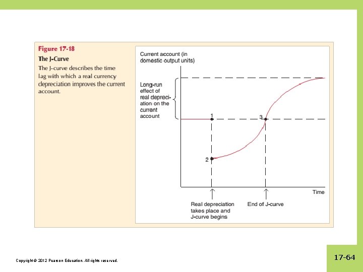
Gradual Trade Flow Adjustment and Current Account Dynamics • An important assumption underlying the DD-AA model is that, other things equal, a real depreciation of the home currency immediately improves the current account. • In reality, however current account adjusts only gradually to exchange rate changes. • The time path of current account presents J-curve pattern corresponding to a real depreciation: initially worsens and afterward gradually improves. Copyright © 2012 Pearson Education. All rights reserved. 17 -63

Copyright © 2012 Pearson Education. All rights reserved. 17 -64

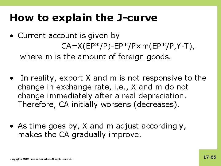
How to explain the J-curve • Current account is given by CA=X(EP*/P)-EP*/P×m(EP*/P, Y-T), where m is the amount of foreign goods. • In reality, export X and m is not responsive to the change in exchange rate, i. e. , X and m do not change immediately after a real depreciation. Therefore, CA initially worsens (decreases). • As time goes by, X and m adjust accordingly, makes the CA gradually improve. Copyright © 2012 Pearson Education. All rights reserved. 17 -65

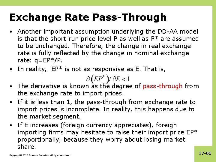
Exchange Rate Pass-Through • Another important assumption underlying the DD-AA model is that the short-run price level P as well as P* are assumed to be unchanged. Therefore, the change in real exchange rate is fully reflected by the change in nominal exchange rate: q=EP*/P. • In reality, EP* is not as responsive as E. That is, • The derivative is known as the degree of pass-through from the exchange rate to import prices. • If it is less than 1, the pass-through from exchange rate to import prices is incomplete. In reality, this happens due to the market segment. • If E increases (foreign currency appreciates), foreign importing firms may hesitate to raise their import price EP* proportionally, because they worry about losing market share. Copyright © 2012 Pearson Education. All rights reserved. 17 -66

The Liquidity Trap • A liquidity trap is a trap because once an economy’s nominal interest rate falls to zero, the central bank cannot reduce it further by increasing the money supply (that is, by increasing the economy’s liquidity). • It worries makers of macroeconomic policy, who are trapped in a situation where they may no longer be able to steer the economy through conventional monetary expansion. • In the liquidity trap, Interest Parity condition implies R=0=R*+(Ee-E)/E. or E=Ee /(1 -R*) which is constant. Copyright © 2012 Pearson Education. All rights reserved. 17 -67

The Liquidity Trap (Cont. ) Copyright © 2012 Pearson Education. All rights reserved. 17 -68

The Liquidity Trap (Cont. ) • Monetary expansion has no effect on output or the exchange rate. This is the sense in which the economy is “trapped”. • Why? • The above result relies on the assumption that expected exchange rate is fixed. If Ee changes, monetary expansion may have effect on the output and the exchange rate, because higher Ee shifts the AA curve up and pull the economy out of the trap. • Another way to stimulate the economy under the liquidity trap is to conduct unconventional montary policy, e. g. Quantitative Easing (QE). Copyright © 2012 Pearson Education. All rights reserved. 17 -69

Summary 1. Aggregate demand is influenced by disposable income and the real exchange rate. 2. The DD curve shows combinations of exchange rates and output where aggregate demand = aggregate output. 3. The AA curve shows combinations of exchange rates and output where the foreign exchange markets and money market are in equilibrium. Copyright © 2012 Pearson Education. All rights reserved. 17 -70

Summary (cont. ) 4. In the DD-AA model, we assume that a depreciation of the domestic currency leads to an increase in the current account and aggregate demand. 5. But reality is more complicated, and the J-curve shows that the value effect at first dominates the volume effect. Copyright © 2012 Pearson Education. All rights reserved. 17 -71

Summary (cont. ) 6. A temporary increase in the money supply is predicted to increase output and depreciate the domestic currency. 7. A permanent increase does both to a larger degree in the short run, but in the long run output returns to its normal level. 8. A temporary increase in government purchases is predicted to increase output and appreciate the domestic currency. 9. A permanent increase in government purchases is predicted to completely crowd out net exports, and therefore to have no effect on output. Copyright © 2012 Pearson Education. All rights reserved. 17 -72