Chapter 17 Numerical Integration Formulas Graphical Representation of

Chapter 17 Numerical Integration Formulas

Graphical Representation of Integral = area under the curve Use of a grid to approximate an integral

Use of strips to approximate an integral

Numerical Integration Survey of land area of an irregular lot Cross-sectional area and volume flowrate in a river Net force against a skyscraper

Pressure Force on a Dam Water exerting pressure on the upstream face of a dam: (a) side view showing force increasing linearly with depth; (b) front view showing width of dam in meters. p = gh = h

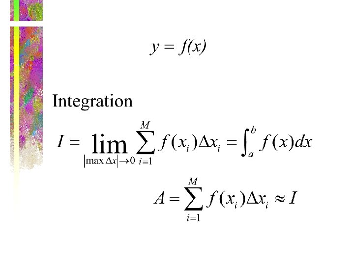
Integration Ø Weighted sum of functional values at discrete points Ø Newton-Cotes closed or open formulae -- evenly spaced points Ø Approximate the function by Lagrange interpolation polynomial Ø Integration of a simple interpolation polynomial Ø Guassian Quadratures Ø Richardson extrapolation and Romberg integration

Basic Numerical Integration Ø Weighted sum of function values f(x) x 0 x 1 xn-1 xn x

Numerical Integration • Idea is to do integral in small parts, like the way you first learned integration - a summation • Numerical methods just try to make it faster and more accurate

Numerical integration Newton-Cotes formulas - based on idea Ø Approximate f(x) by a polynomial

Ø fn (x) can be linear Ø fn (x) can be quadratic

Ø fn (x) can also be cubic or other higher-order polynomials

Ø Polynomial can be piecewise over the data

Numerical Integration Ø Newton-Cotes Closed Formulae -- Use both end points q q q Trapezoidal Rule : Linear Simpson’s 1/3 -Rule : Quadratic Simpson’s 3/8 -Rule : Cubic Boole’s Rule : Fourth-order* Higher-order methods* Ø Newton-Cotes Open Formulae -- Use only interior points q q midpoint rule Higher-order methods

Closed and Open Formulae (a) End points are known (b) Extrapolation

Trapezoidal Rule • Straight-line approximation f(x) L(x) x 0 x 1 x

Trapezoidal Rule • Lagrange interpolation

Example: Trapezoidal Rule • Evaluate the integral • Exact solution • Trapezoidal Rule

Better Numerical Integration Ø Composite integration Ø Multiple applications of Newton-Cotes formulae Ø Composite Trapezoidal Rule Ø Composite Simpson’s Rule Ø Richardson Extrapolation Ø Romberg integration

Apply trapezoidal rule to multiple segments over integration limits Two segments Three segments Four segments Many segments

Multiple Applications of Trapezoidal Rule

Composite Trapezoidal Rule f(x) x 0 h x 1 h x 2 h x 3 h x 4 x

Trapezoidal Rule Ø Truncation error (single application) Ø Exact if the function is linear ( f = 0) Ø Use multiple applications to reduce the truncation error Approximate error

Composite Trapezoidal Rule function f = example 1(x) % a = 0, b = pi f=x. ^2. *sin(2*x);

Composite Trapezoidal Rule » » » I a=0; b=pi; dx=(b-a)/100; x=a: dx: b; y=example 1(x); I=trap('example 1', a, b, 1) = -3. 7970 e-015 » I=trap('example 1', a, b, 2) I = -1. 4239 e-015 » I=trap('example 1', a, b, 4) I = -3. 8758 » I=trap('example 1', a, b, 8) I = -4. 6785 » I=trap('example 1', a, b, 16) I = -4. 8712 » I=trap('example 1', a, b, 32) I = -4. 9189 » I=trap('example 1', a, b, 64) I = -4. 9308 » I=trap('example 1', a, b, 128) I = -4. 9338 » I=trap('example 1', a, b, 256) I = -4. 9346 » I=trap('example 1', a, b, 512) I = -4. 9347 » I=trap('example 1', a, b, 1024) I = -4. 9348 » Q=quad 8('example 1', a, b) Q = -4. 9348 MATLAB function

n=2 I = -1. 4239 e-15 Exact = -4. 9348

n=4 I = -3. 8758 Exact = -4. 9348

n=8 I = -4. 6785 Exact = -4. 9348

n = 16 I = -4. 8712 Exact = -4. 9348

Composite Trapezoidal Rule • Evaluate the integral

Composite Trapezoidal Rule » » » » x=0: 0. 04: 4; y=example 2(x); x 1=0: 4: 4; y 1=example 2(x 1); x 2=0: 2: 4; y 2=example 2(x 2); x 3=0: 1: 4; y 3=example 2(x 3); x 4=0: 0. 5: 4; y 4=example 2(x 4); H=plot(x, y, x 1, y 1, 'g-*', x 2, y 2, 'r-s', x 3, y 3, 'c-o', x 4, y 4, 'm-d'); set(H, 'Line. Width', 3, 'Marker. Size', 12); xlabel('x'); ylabel('y'); title('f(x) = x exp(2 x)'); » I=trap('example 2', 0, 4, 1) I = 2. 3848 e+004 » I=trap('example 2', 0, 4, 2) I = 1. 2142 e+004 » I=trap('example 2', 0, 4, 4) I = 7. 2888 e+003 » I=trap('example 2', 0, 4, 8) I = 5. 7648 e+003 » I=trap('example 2', 0, 4, 16) I = 5. 3559 e+003

Composite Trapezoidal Rule

Simpson’s 1/3 -Rule • Approximate the function by a parabola L(x) f(x) x 0 h x 1 h x 2 x

Simpson’s 1/3 -Rule

Simpson’s 1/3 -Rule

Composite Simpson’s Rule Piecewise Quadratic approximations f(x) …. . . x 0 h x 1 h x 2 h x 3 h x 4 xn-2 xn-1 xn x

Composite Simpson’s 1/3 Rule Ø Applicable only if the number of segments is even

Composite Simpson’s 1/3 Rule Ø Applicable only if the number of segments is even Ø Substitute Simpson’s 1/3 rule for each integral Ø For uniform spacing (equal segments)

Simpson’s 1/3 Rule Ø Truncation error (single application) Ø Exact up to cubic polynomial ( f (4)= 0) Ø Approximate error for (n/2) multiple applications

Composite Simpson’s 1/3 Rule Ø Evaluate the integral • n = 2, h = 2 • n = 4, h = 1

Simpson’s 3/8 -Rule Ø Approximate by a cubic polynomial L(x) x 0 h f(x) x 1 h x 2 h x 3 x

Simpson’s 3/8 -Rule Ø Truncation error

Example: Simpson’s Rules Ø Evaluate the integral Ø Simpson’s 1/3 -Rule Ø Simpson’s 3/8 -Rule

Composite Simpson’s 1/3 Rule function I = Simp(f, a, b, n) % integral of f using composite Simpson rule % n must be even h = (b - a)/n; S = feval(f, a); for i = 1 : 2 : n-1 x(i) = a + h*i; S = S + 4*feval(f, x(i)); end for i = 2 : n-2 x(i) = a + h*i; S = S + 2*feval(f, x(i)); end S = S + feval(f, b); I = h*S/3;

Simpson’s 1/3 Rule

Composite Simpson’s 1/3 Rule

» » » » I » I » Q x=0: 0. 04: 4; y=example(x); x 1=0: 2: 4; y 1=example(x 1); c=Lagrange_coef(x 1, y 1); p 1=Lagrange_eval(x, x 1, c); H=plot(x, y, x 1, y 1, 'r*', x, p 1, 'r'); xlabel('x'); ylabel('y'); title('f(x) = x*exp(2 x)'); set(H, 'Line. Width', 3, 'Marker. Size', 12); x 2=0: 1: 4; y 2=example(x 2); c=Lagrange_coef(x 2, y 2); p 2=Lagrange_eval(x, x 2, c); H=plot(x, y, x 2, y 2, 'r*', x, p 2, 'r'); xlabel('x'); ylabel('y'); title('f(x) = x*exp(2 x)'); set(H, 'Line. Width', 3, 'Marker. Size', 12); I=Simp('example', 0, 4, 2) = 8. 2404 e+003 I=Simp('example', 0, 4, 4) = 5. 6710 e+003 I=Simp('example', 0, 4, 8) = 5. 2568 e+003 I=Simp('example', 0, 4, 16) = 5. 2197 e+003 Q=Quad 8('example', 0, 4) = 5. 2169 e+003 n=2 n=4 n=8 n = 16 MATLAB fun

Multiple applications of Simpson’s rule with odd number of intervals Hybrid Simpson’s 1/3 & 3/8 rules

Newton-Cotes Closed Integration Formulae

Composite Trapezoidal Rule with Unequal Segments Ø Evaluate the integral Ø h 1 = 2, h 2 = 1, h 3 = 0. 5, h 4 = 0. 5

Trapezoidal Rule for Unequally Spaced Data

MATLAB Function: trapz Ø Z = trapz(x, y) » x=[0 1 1. 5 2. 0 2. 5 3. 0 3. 3 3. 6 3. 8 3. 9 4. 0] x = Columns 1 through 7 0 1. 0000 Columns 8 through 11 3. 6000 3. 8000 » y=x. *exp(2. *x) y = 1. 0 e+004 * Columns 1 through 7 0 0. 0007 Columns 8 through 11 0. 4822 0. 7593 » integr = trapz(x, y) integr = 5. 3651 e+003 1. 5000 2. 0000 3. 9000 4. 0000 0. 0030 0. 0109 0. 9518 1. 1924 2. 5000 3. 0000 3. 3000 0. 0371 0. 1210 0. 2426

Integral of Unevenly-Spaced Data Ø Trapezoidal rule Ø Could also be evaluated with Simpson’s rule for higher accuracy

Composite Simpson’s Rule with Unequal Segments • Evaluate the integral • h 1 = 1. 5, h 2 = 0. 5

Newton-Cotes Open Formula Midpoint Rule (One-point) f(x) a xm b x

Two-point Newton-Cotes Open Formula Ø Approximate by a straight line f(x) x 0 h x 1 h x 2 h x 3 x

Three-point Newton-Cotes Open Formula Ø Approximate by a parabola f(x) x 0 h x 1 h x 2 h x 3 h x 4 x

Newton-Cotes Open Integration Formulae

Double Integral Ø Area under the function surface

Double Integral Ø T(x, y) = 2 xy + 2 x – x 2 – 2 y 2 + 40 Ø Two-segment trapezoidal rule Ø Exact if usingle-segment Simpson’s 1/3 rule (because the function is quadratic in x and y)