Chapter 16 Scheduling Copyright 2015 Mc GrawHill Education

Chapter 16 Scheduling Copyright © 2015 Mc. Graw-Hill Education. All rights reserved. No reproduction or distribution without the prior written consent of Mc. Graw-Hill Education.

Chapter 16: Learning Objectives You should be able to: LO 16. 1 Explain what scheduling involves and the importance of good scheduling LO 16. 2 Compare product and service scheduling hierarchies LO 16. 3 Describe scheduling needs in high-volume systems LO 16. 4 Describe scheduling needs in intermediate-volume systems LO 16. 5 Describe scheduling needs in job shops LO 16. 6 Use and interpret Gantt charts LO 16. 7 Use the assignment method for loading LO 16. 8 Give examples of commonly used priority rules LO 16. 9 Discuss the Theory of Constraints and that approach to scheduling LO 16. 10 Summarize some of the unique problems encountered in service systems, and describe some of the approaches used for scheduling service systems 16 -2

Scheduling: Establishing the timing of the use of equipment, facilities and human activities in an organization Effective scheduling can yield Cost savings Increases in productivity Other benefits LO 16. 1 16 -3

Scheduling Context Scheduling is constrained by multiple system design and operations decisions System capacity Product and/or service design Equipment selection Worker selection and training Aggregate planning and master scheduling LO 16. 1 16 -4

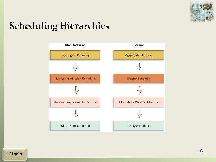
Scheduling Hierarchies LO 16. 2 16 -5

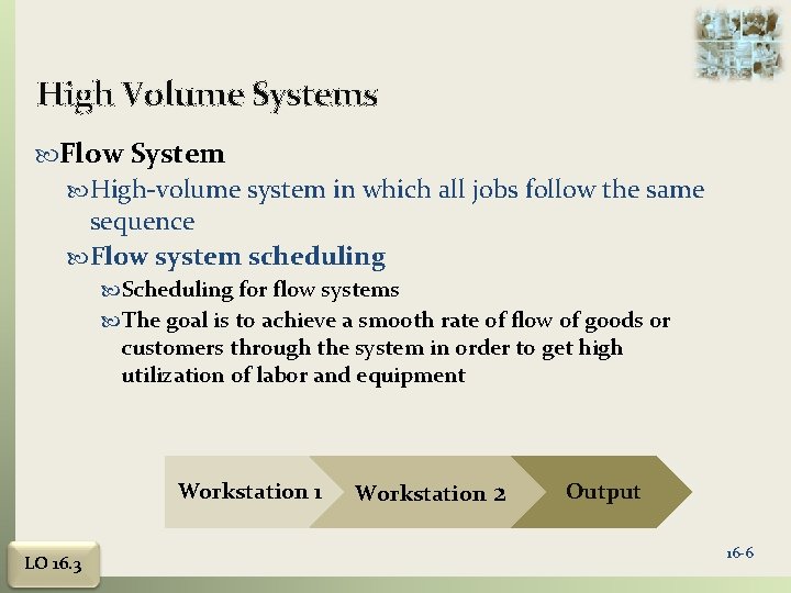
High Volume Systems Flow System High-volume system in which all jobs follow the same sequence Flow system scheduling Scheduling for flow systems The goal is to achieve a smooth rate of flow of goods or customers through the system in order to get high utilization of labor and equipment Workstation 1 LO 16. 3 Workstation 2 Output 16 -6

High-Volume: Scheduling Difficulties Few flow systems are entirely dedicated to a single product or service Each product change requires Slightly different inputs of parts Slightly different materials Slightly different processing requirements that must be scheduled into the line Need to avoid excessive inventory buildup Disruptions may result in less-than-desired output LO 16. 3 16 -7

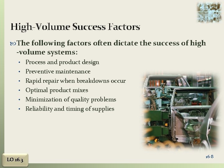
High-Volume Success Factors The following factors often dictate the success of high -volume systems: • Process and product design • Preventive maintenance • Rapid repair when breakdowns occur • Optimal product mixes • Minimization of quality problems • Reliability and timing of supplies LO 16. 3 16 -8

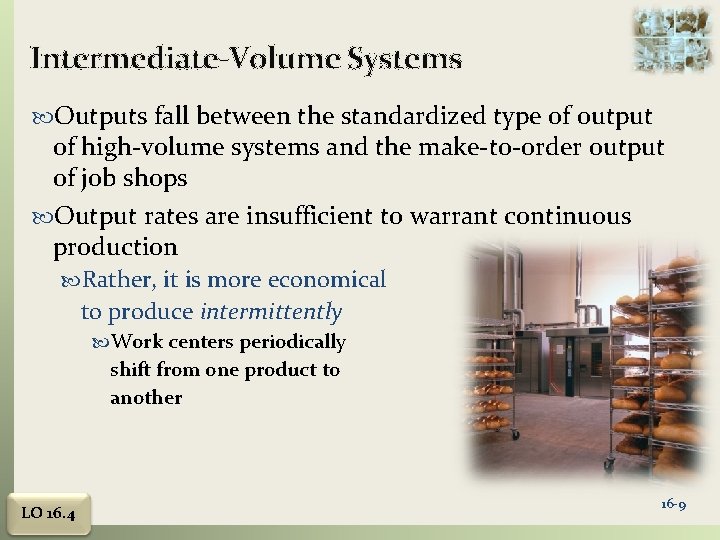
Intermediate-Volume Systems Outputs fall between the standardized type of output of high-volume systems and the make-to-order output of job shops Output rates are insufficient to warrant continuous production Rather, it is more economical to produce intermittently Work centers periodically shift from one product to another LO 16. 4 16 -9

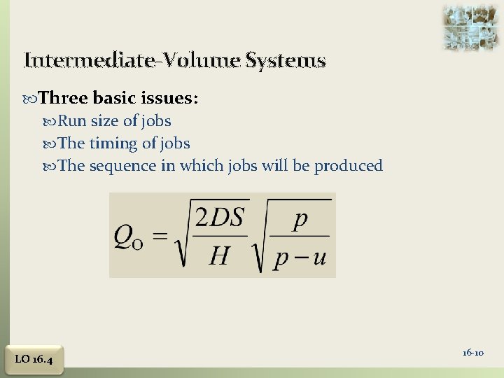
Intermediate-Volume Systems Three basic issues: Run size of jobs The timing of jobs The sequence in which jobs will be produced LO 16. 4 16 -10

Intermediate-Volume Systems Important considerations Setup cost Usage is not always as smooth as assumed in the economic lot size model Alternative scheduling approach Base production on a master schedule developed from customer orders and forecasted demand LO 16. 4 16 -11

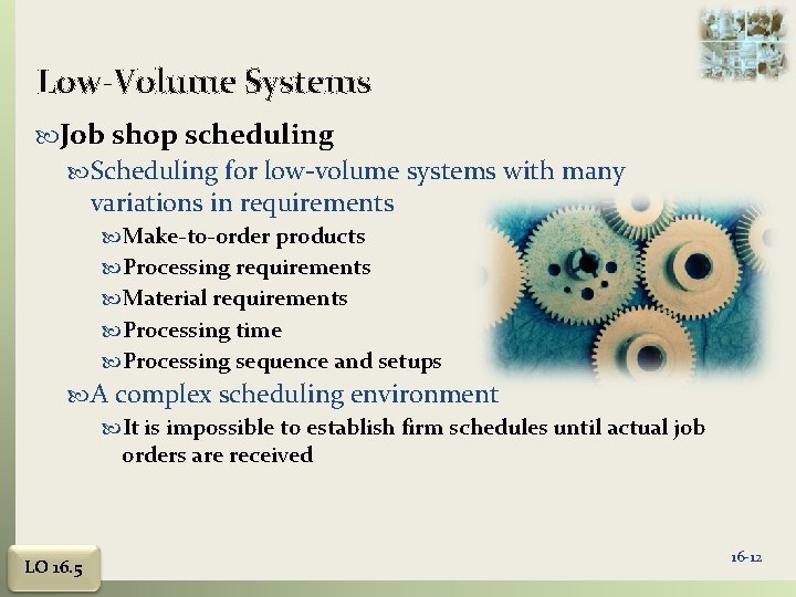
Low-Volume Systems Job shop scheduling Scheduling for low-volume systems with many variations in requirements Make-to-order products Processing requirements Material requirements Processing time Processing sequence and setups A complex scheduling environment It is impossible to establish firm schedules until actual job orders are received LO 16. 5 16 -12

Low-Volume Systems: Loading the assignment of jobs to processing centers Gantt chart Used as a visual aid for loading and scheduling purposes Purpose of the Gantt chart is to organize and visually display the actual or intended use of resources in a time framework Managers may use the charts for trial-and-error schedule development to get an idea of what different arrangements would involve LO 16. 5 16 -13

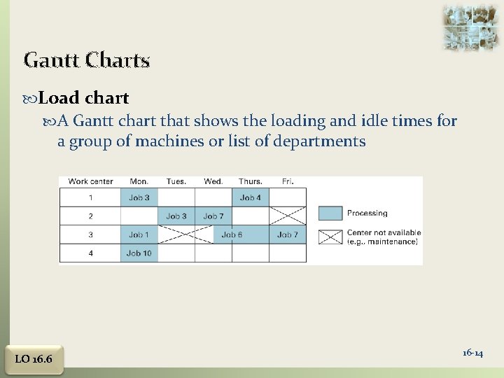
Gantt Charts Load chart A Gantt chart that shows the loading and idle times for a group of machines or list of departments LO 16. 6 16 -14

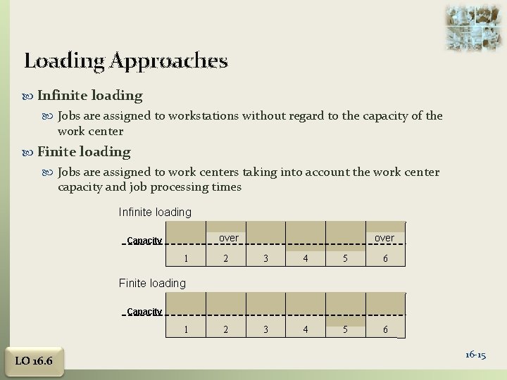
Loading Approaches Infinite loading Jobs are assigned to workstations without regard to the capacity of the work center Finite loading Jobs are assigned to work centers taking into account the work center capacity and job processing times Infinite loading over Capacity 1 over 2 3 4 5 6 Finite loading Capacity 1 LO 16. 6 16 -15

Scheduling Approaches · · Forward scheduling · Scheduling ahead from some point in time. · Used when the question is: · “How long will it take to complete this job? Backward scheduling · Scheduling backwards from some due date · Used when the question is: · “When is the latest this job can be started and still be completed on time? ” LO 16. 6 16 -16

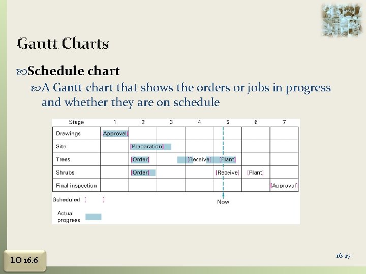
Gantt Charts Schedule chart A Gantt chart that shows the orders or jobs in progress and whether they are on schedule LO 16. 6 16 -17

Assignment model A linear programming model for optimal assignment of tasks and resources Hungarian method Method of assigning jobs by a one-for-one matching to identify the lowest cost solution LO 16. 7 16 -18

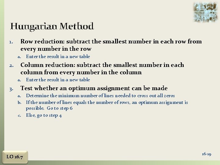
Hungarian Method 1. Row reduction: subtract the smallest number in each row from every number in the row a. 2. Column reduction: subtract the smallest number in each column from every number in the column a. 3. Enter the result in a new table Test whether an optimum assignment can be made Determine the minimum number of lines needed to cross out all zeros b. If the number of lines equals the number of rows, an optimum assignment is possible. Go to step 6 c. Else, go to step 4 a. LO 16. 7 16 -19

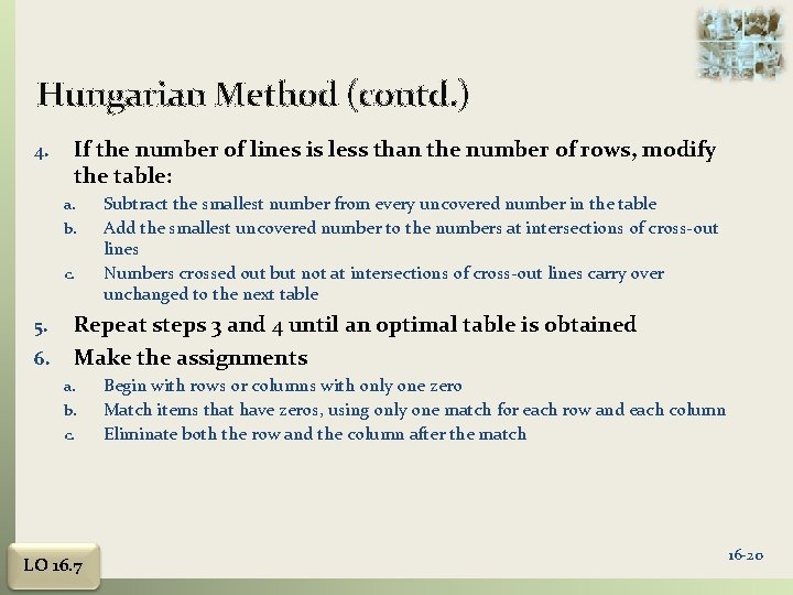
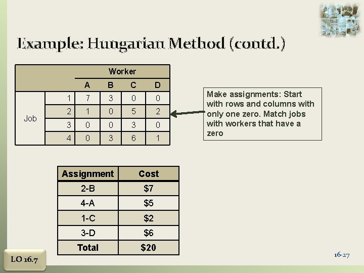
Hungarian Method (contd. ) 4. If the number of lines is less than the number of rows, modify the table: a. b. c. 5. 6. Subtract the smallest number from every uncovered number in the table Add the smallest uncovered number to the numbers at intersections of cross-out lines Numbers crossed out but not at intersections of cross-out lines carry over unchanged to the next table Repeat steps 3 and 4 until an optimal table is obtained Make the assignments a. b. c. LO 16. 7 Begin with rows or columns with only one zero Match items that have zeros, using only one match for each row and each column Eliminate both the row and the column after the match 16 -20

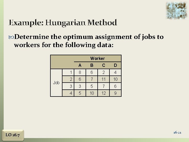
Example: Hungarian Method Determine the optimum assignment of jobs to workers for the following data: Worker Job LO 16. 7 A B C D 1 8 6 2 4 2 6 7 11 10 3 3 5 7 6 4 5 10 12 9 16 -21

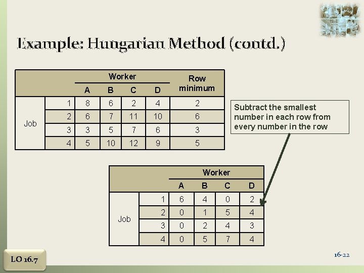
Example: Hungarian Method (contd. ) Worker Job A B C D Row minimum 1 8 6 2 4 2 2 6 7 11 10 6 3 3 5 7 6 3 4 5 10 12 9 5 Subtract the smallest number in each row from every number in the row Worker Job LO 16. 7 A B C D 1 6 4 0 2 2 0 1 5 4 3 0 2 4 3 4 0 5 7 4 16 -22

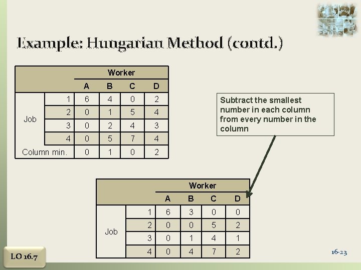
Example: Hungarian Method (contd. ) Worker Job A B C D 1 6 4 0 2 2 0 1 5 4 3 0 2 4 3 4 0 5 7 4 0 1 0 2 Column min. Subtract the smallest number in each column from every number in the column Worker Job LO 16. 7 A B C D 1 6 3 0 0 2 0 0 5 2 3 0 1 4 0 4 7 2 16 -23

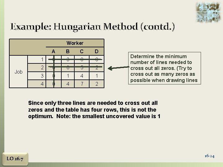
Example: Hungarian Method (contd. ) Worker Job A B C D 1 6 3 0 0 2 0 0 5 2 3 0 1 4 0 4 7 2 Determine the minimum number of lines needed to cross out all zeros. (Try to cross out as many zeros as possible when drawing lines Since only three lines are needed to cross out all zeros and the table has four rows, this is not the optimum. Note: the smallest uncovered value is 1 LO 16. 7 16 -24

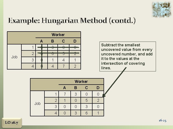
Example: Hungarian Method (contd. ) Worker Job A B C D 1 6 3 0 0 2 0 0 5 2 3 0 1 4 0 4 7 2 Subtract the smallest uncovered value from every uncovered number, and add it to the values at the intersection of covering lines. Worker Job LO 16. 7 A B C D 1 7 3 0 0 2 1 0 5 2 3 0 0 3 0 4 0 3 6 1 16 -25

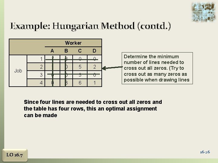
Example: Hungarian Method (contd. ) Worker Job A B C D 1 7 3 0 0 2 1 0 5 2 3 0 0 3 0 4 0 3 6 1 Determine the minimum number of lines needed to cross out all zeros. (Try to cross out as many zeros as possible when drawing lines Since four lines are needed to cross out all zeros and the table has four rows, this an optimal assignment can be made LO 16. 7 16 -26

Example: Hungarian Method (contd. ) Worker Job LO 16. 7 A B C D 1 7 3 0 0 2 1 0 5 2 3 0 0 3 0 4 0 3 6 1 Assignment Cost 2 -B $7 4 -A $5 1 -C $2 3 -D $6 Total $20 Make assignments: Start with rows and columns with only one zero. Match jobs with workers that have a zero 16 -27

Sequencing Problem Sequencing Determine the order in which jobs at a work center will be processed Priority rules Simple heuristics used to select the order in which jobs will be processed The rules generally assume that job setup cost and time are independent of processing sequence Job time Time needed for setup and processing of a job LO 16. 8 16 -28

Order-Sequencing Problems We want to determine the sequence in which we will process a group of waiting orders at a work center. Many different sequencing rules can be followed in setting the priorities among orders. There are numerous criteria for evaluating the effectiveness of the sequencing rules. 16 -29

Priority Rules: Assumptions The set of jobs is known; no new orders arrive after processing begins and no jobs are canceled Setup time is independent of processing sequence Setup time is deterministic Processing times are deterministic There will be no interruptions in processing such as machine breakdowns or accidents LO 16. 8 16 -30

Order-Sequencing Rules First-Come First-Served (FCFS) Next job to process is the one that arrived first among the waiting jobs Shortest Processing Time (SPT) Next job to process is the one with the shortest processing time among the waiting jobs Earliest Due Date (EDD) Next job to process is the one with the earliest due (promised finished) date among the waiting jobs 16 -31

Order-Sequencing Rules Least Slack (LS) Next job to process is the one with the least [time to due date minus total remaining processing time] among the waiting jobs Critical Ratio (CR) Next job to process is the one with the least [time to due date divided by total remaining processing time] among the waiting jobs Least Changeover Cost (LCC) Sequence the waiting jobs such that total machine changeover cost is minimized 16 -32

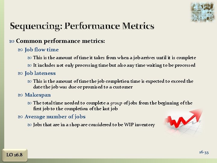
Sequencing: Performance Metrics Common performance metrics: Job flow time This is the amount of time it takes from when a job arrives until it is complete It includes not only processing time but also any time waiting to be processed Job lateness This is the amount of time the job completion time is expected to exceed the date the job was due or promised to a customer Makespan The total time needed to complete a group of jobs from the beginning of the first job to the completion of the last job Average number of jobs Jobs that are in a shop are considered to be WIP inventory LO 16. 8 16 -33

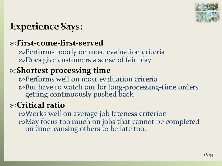
Experience Says: First-come-first-served Performs poorly on most evaluation criteria Does give customers a sense of fair play Shortest processing time Performs well on most evaluation criteria But have to watch out for long-processing-time orders getting continuously pushed back Critical ratio Works well on average job lateness criterion May focus too much on jobs that cannot be completed on time, causing others to be late too. 16 -34

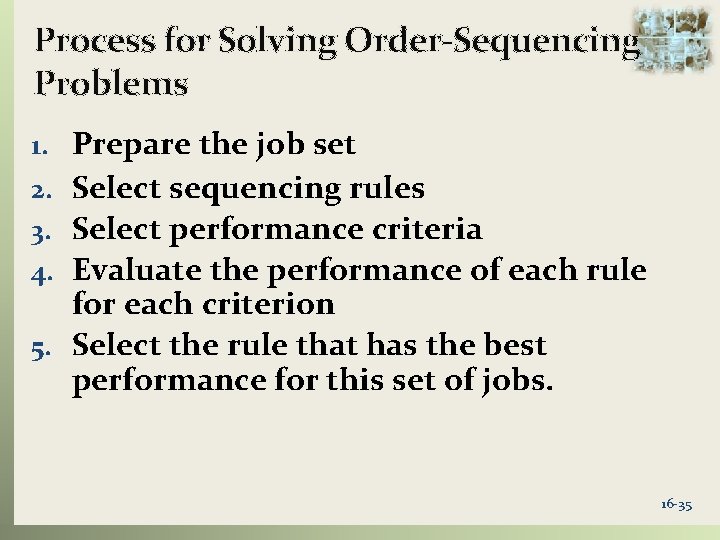
Process for Solving Order-Sequencing Problems 1. Prepare the job set 2. Select sequencing rules 3. Select performance criteria 4. Evaluate the performance of each rule for each criterion 5. Select the rule that has the best performance for this set of jobs. 16 -35

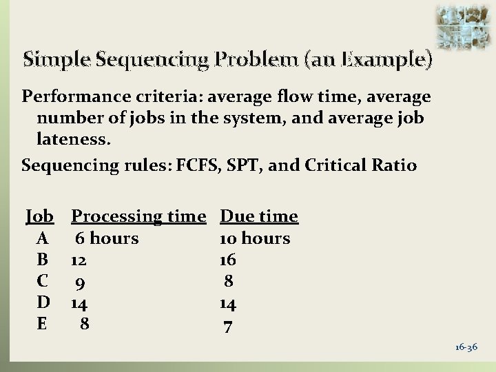
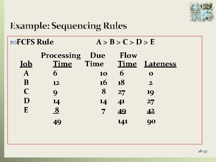
Simple Sequencing Problem (an Example) Performance criteria: average flow time, average number of jobs in the system, and average job lateness. Sequencing rules: FCFS, SPT, and Critical Ratio Job Processing time A 6 hours B 12 C 9 D 14 E 8 Due time 10 hours 16 8 14 7 16 -36

Example: Sequencing Rules FCFS Rule Job A B C D E A>B>C>D>E Processing Due Time 6 10 12 16 9 8 14 14 8 7 49 Flow Time Lateness 6 0 18 2 27 19 41 27 49 42 141 90 16 -37

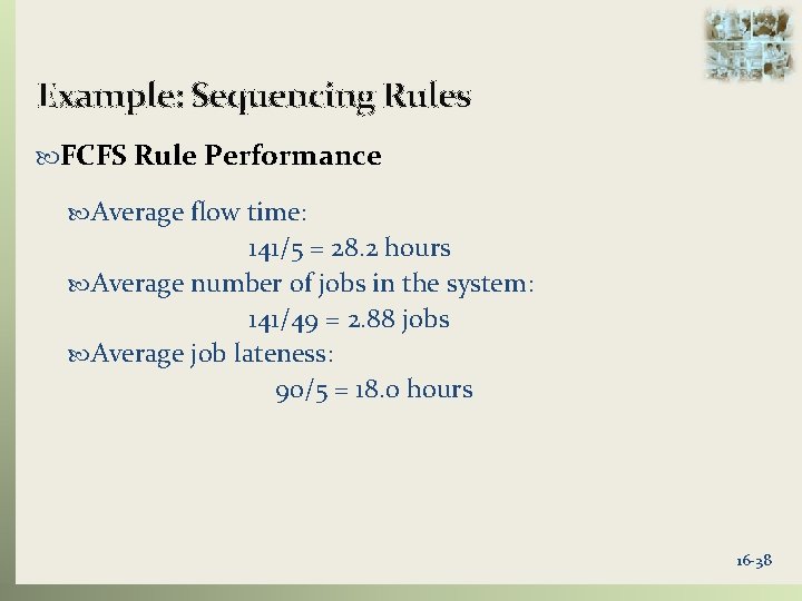
Example: Sequencing Rules FCFS Rule Performance Average flow time: 141/5 = 28. 2 hours Average number of jobs in the system: 141/49 = 2. 88 jobs Average job lateness: 90/5 = 18. 0 hours 16 -38

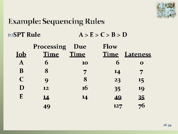
Example: Sequencing Rules SPT Rule Job A B C D E A>E>C>B>D Processing Due Time 6 10 8 7 9 8 12 16 14 14 49 Flow Time Lateness 6 0 14 7 23 15 35 19 49 35 127 76 16 -39

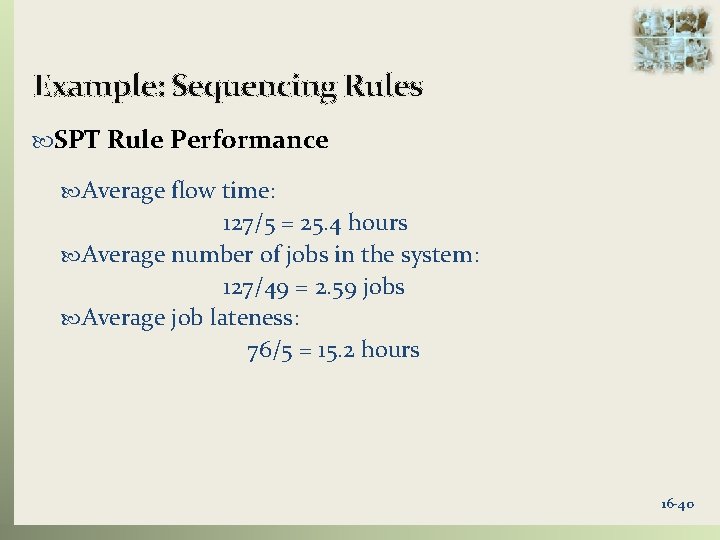
Example: Sequencing Rules SPT Rule Performance Average flow time: 127/5 = 25. 4 hours Average number of jobs in the system: 127/49 = 2. 59 jobs Average job lateness: 76/5 = 15. 2 hours 16 -40

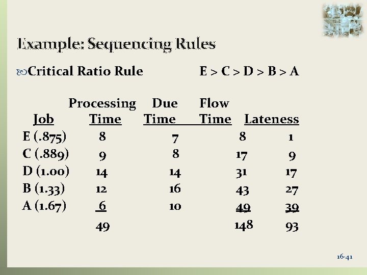
Example: Sequencing Rules Critical Ratio Rule Processing Due Job Time E (. 875) 8 7 C (. 889) 9 8 D (1. 00) 14 14 B (1. 33) 12 16 A (1. 67) 6 10 49 E>C>D>B>A Flow Time Lateness 8 1 17 9 31 17 43 27 49 39 148 93 16 -41

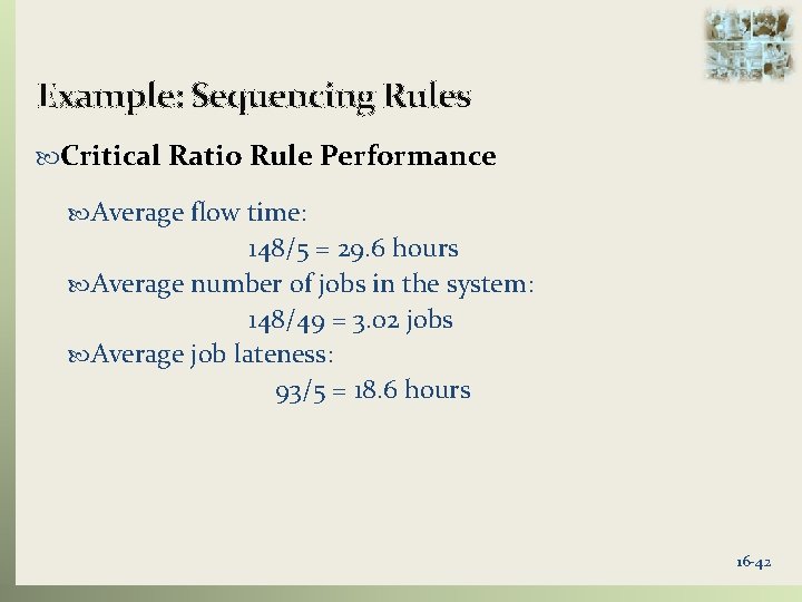
Example: Sequencing Rules Critical Ratio Rule Performance Average flow time: 148/5 = 29. 6 hours Average number of jobs in the system: 148/49 = 3. 02 jobs Average job lateness: 93/5 = 18. 6 hours 16 -42

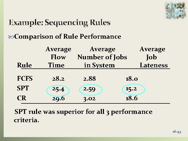
Example: Sequencing Rules Comparison of Rule Performance Rule FCFS SPT CR Average Flow Number of Jobs Time in System 28. 2 25. 4 29. 6 2. 88 2. 59 3. 02 Average Job Lateness 18. 0 15. 2 18. 6 SPT rule was superior for all 3 performance criteria. 16 -43

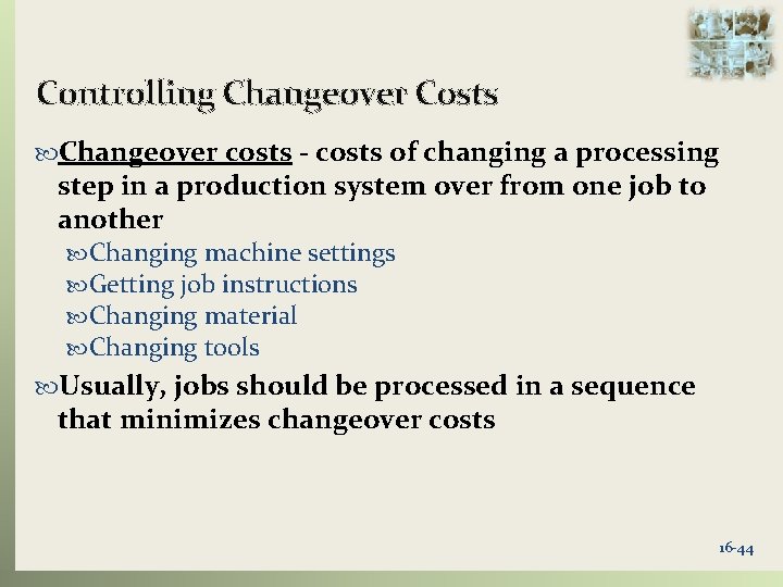
Controlling Changeover Costs Changeover costs - costs of changing a processing step in a production system over from one job to another Changing machine settings Getting job instructions Changing material Changing tools Usually, jobs should be processed in a sequence that minimizes changeover costs 16 -44

Controlling Changeover Costs Job Sequencing Heuristic First, select the lowest changeover cost among all changeovers (this establishes the first two jobs in the sequence) The next job to be selected will have the lowest changeover cost among the remaining jobs that follow the previously selected job 16 -45

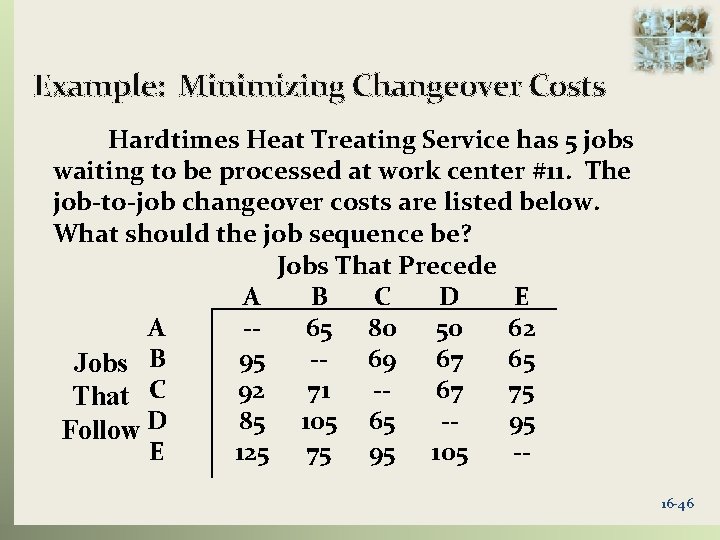
Example: Minimizing Changeover Costs Hardtimes Heat Treating Service has 5 jobs waiting to be processed at work center #11. The job-to-job changeover costs are listed below. What should the job sequence be? Jobs That Precede A B C D E A -65 80 50 62 95 -69 67 65 Jobs B 92 71 -67 75 That C 85 105 65 -95 Follow D E 125 75 95 105 -16 -46

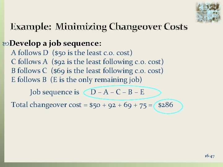
Example: Minimizing Changeover Costs Develop a job sequence: A follows D ($50 is the least c. o. cost) C follows A ($92 is the least following c. o. cost) B follows C ($69 is the least following c. o. cost) E follows B (E is the only remaining job) Job sequence is D–A–C–B–E Total changeover cost = $50 + 92 + 69 + 75 = $286 16 -47

Two Work Center Sequencing (Flow Shop) Johnson’s Rule Technique for minimizing makespan for a group of jobs to be processed on two machines or at two work centers. Minimizes total idle time Several conditions must be satisfied LO 16. 8 16 -48

Johnson’s Rule Conditions Job time must be known and constant for each job at the work center Job times must be independent of sequence Jobs must follow same two-step sequence All jobs must be completed at the first work center before moving to second work center LO 16. 8 16 -49

Johnson’s Rule: Optimum Sequence 1. List the jobs and their times at each work center 2. Select the job with the shortest time a. If the shortest time is at the first work center, schedule that job first b. If the shortest time is at the second work center, schedule the job last. c. Break ties arbitrarily 3. Eliminate the job from further consideration 4. Repeat steps 2 and 3, working toward the center of the sequence, until all jobs have been scheduled LO 16. 8 16 -50

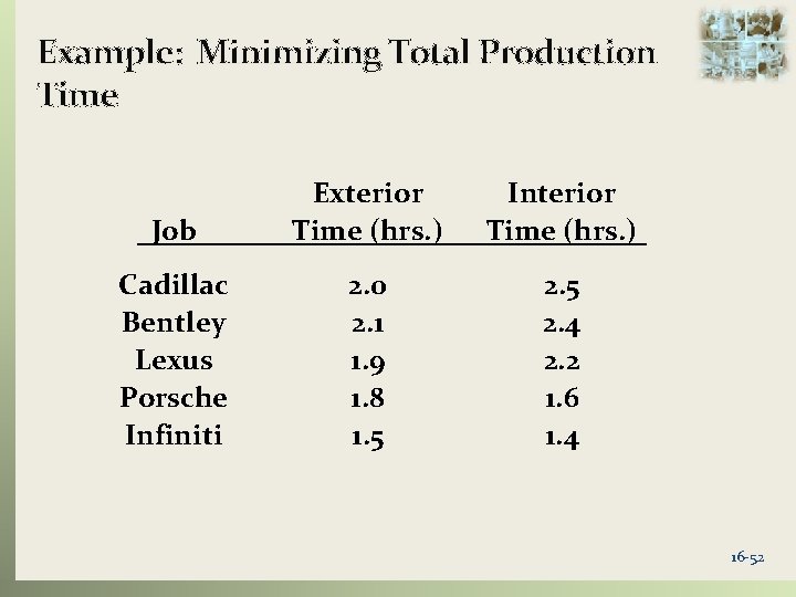
Example: Minimizing Total Production Time It is early Saturday morning and The Finest Detail has five automobiles waiting for detailing service. Each vehicle goes through a thorough exterior wash/wax process and then an interior vacuum/shampoo/polish process. The entire detailing crew must stay until the last vehicle is completed. If the five vehicles are sequenced so that the total processing time is minimized, when can the crew go home. They will start the first vehicle at 7: 30 a. m. Time estimates are shown on the next slide. 16 -51

Example: Minimizing Total Production Time Job Exterior Time (hrs. ) Interior Time (hrs. ) Cadillac Bentley Lexus Porsche Infiniti 2. 0 2. 1 1. 9 1. 8 1. 5 2. 4 2. 2 1. 6 1. 4 16 -52

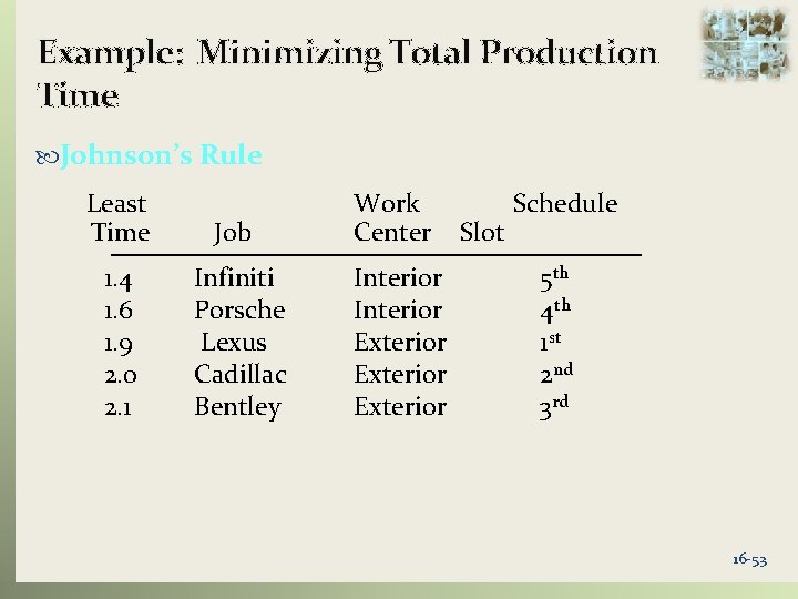
Example: Minimizing Total Production Time Johnson’s Rule Least Time Job Work Center 1. 4 1. 6 1. 9 2. 0 2. 1 Infiniti Porsche Lexus Cadillac Bentley Interior Exterior Slot Schedule 5 th 4 th 1 st 2 nd 3 rd 16 -53

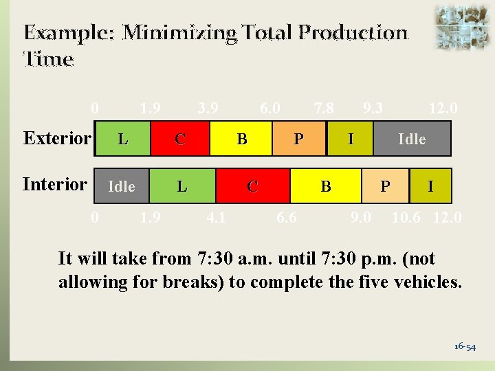
Example: Minimizing Total Production Time 0 Exterior 1. 9 L C Interior Idle 0 3. 9 B L 1. 9 6. 0 7. 8 P C 4. 1 9. 3 I B 6. 6 Idle P 9. 0 12. 0 I 10. 6 12. 0 It will take from 7: 30 a. m. until 7: 30 p. m. (not allowing for breaks) to complete the five vehicles. 16 -54

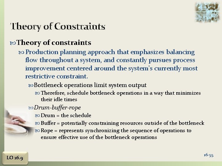
Theory of Constraints Theory of constraints Production planning approach that emphasizes balancing flow throughout a system, and constantly pursues process improvement centered around the system’s currently most restrictive constraint. Bottleneck operations limit system output Therefore, schedule bottleneck operations in a way that minimizes their idle times Drum-buffer-rope Drum = the schedule Buffer = potentially constraining resources outside of the bottleneck Rope = represents synchronizing the sequence of operations to ensure effective use of the bottleneck operations LO 16. 9 16 -55

Theory of Constraints (contd. ) Varying batch sizes to achieve greatest output of bottleneck operations Process batch The economical quantity to produce upon the activation of a given operation Transfer batch The quantity to be transported from one operation to another, assumed to be smaller than the first operation’s process batch LO 16. 9 16 -56

Theory of Constraints (contd. ) Improving bottleneck operations: 1. Determine what is constraining the operation 2. Exploit the constraint (i. e. , make sure the constraining resource is used to its maximum) 3. Subordinate everything to the constraint (i. e. , focus on the constraint) 4. Determine how to overcome (eliminate) the constraint 5. Repeat the process for the next highest constraint LO 16. 9 16 -57

Theory of Constraints: Metrics Three important theory of constraints metrics: Throughput The rate at which the system generates money through sales Inventory represents money tied up in goods and materials used in a process Operating expense All the money the system spends to convert inventory into throughput: this includes utilities, scrap, depreciation, and so on LO 16. 9 16 -58

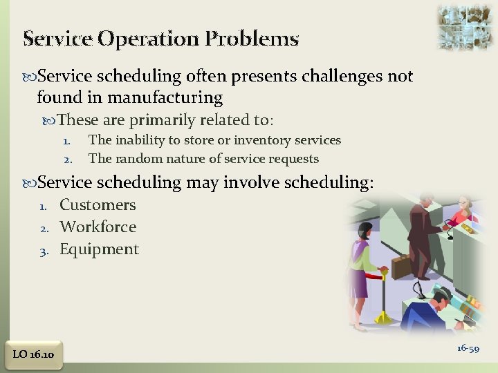
Service Operation Problems Service scheduling often presents challenges not found in manufacturing These are primarily related to: 1. The inability to store or inventory services 2. The random nature of service requests Service scheduling may involve scheduling: 1. 2. 3. LO 16. 10 Customers Workforce Equipment 16 -59

Scheduling Service Operations Scheduling customers: Demand Management Appointment systems Controls customer arrivals for service Reservation systems Enable service systems to formulate a fairly accurate estimate demand on the system for a given time period Scheduling the workforce: Capacity Management Cyclical Scheduling Employees are assigned to work shifts or time slots, and have days off, on a repeating basis LO 16. 10 16 -60