Chapter 16 Chi Squared Tests 16 1 Introduction

Chapter 16 Chi Squared Tests

16. 1 Introduction • Two statistical techniques are presented, to analyze nominal data. – A goodness-of-fit test for the multinomial experiment. – A contingency table test of independence. • Both tests use the c 2 as the sampling distribution of the test statistic.

16. 2 Chi-Squared Goodness-of. Fit Test • The hypothesis tested involves the probabilities p 1, p 2, …, pk. of a multinomial distribution. • The multinomial experiment is an extension of the binomial experiment. – There are n independent trials. – The outcome of each trial can be classified into one of k categories, called cells. – The probability pi that the outcome fall into cell i remains constant for each trial. Moreover, p 1 + p 2 + … +pk = 1. – Trials of the experiment are independent

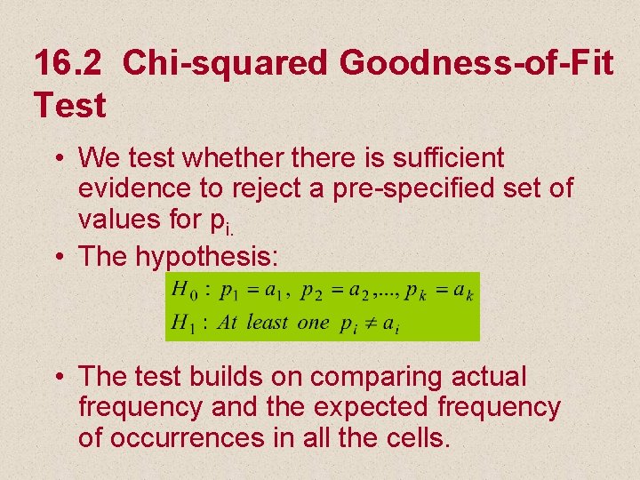
16. 2 Chi-squared Goodness-of-Fit Test • We test whethere is sufficient evidence to reject a pre-specified set of values for pi. • The hypothesis: • The test builds on comparing actual frequency and the expected frequency of occurrences in all the cells.

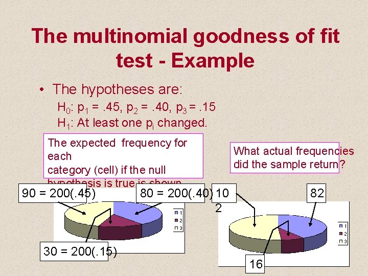
The multinomial goodness of fit test - Example • Example 16. 1 – Two competing companies A and B have enjoy dominant position in the market. The companies conducted aggressive advertising campaigns. – Market shares before the campaigns were: • Company A = 45% • Company B = 40% • Other competitors = 15%.

The multinomial goodness of fit test - Example • Example 16. 1 – continued – To study the effect of the campaign on the market shares, a survey was conducted. – 200 customers were asked to indicate their preference regarding the product advertised. – Survey results: • 102 customers preferred the company A’s product, • 82 customers preferred the company B’s product,

The multinomial goodness of fit test - Example • Example 16. 1 – continued Can we conclude at 5% significance level that the market shares were affected by the advertising campaigns?

The multinomial goodness of fit test - Example • Solution – The population investigated is the brand preferences. – The data are nominal (A, B, or other) – This is a multinomial experiment (three categories). – The question of interest: Are p 1, p 2, and p 3 different after the campaign from their values before the campaign?

The multinomial goodness of fit test - Example • The hypotheses are: H 0: p 1 =. 45, p 2 =. 40, p 3 =. 15 H 1: At least one pi changed. The expected frequency for What actual frequencies each did the sample return? category (cell) if the null hypothesis is true is shown 90 = below: 200(. 45) 80 = 200(. 40) 10 82 2 30 = 200(. 15) 16

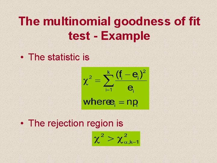
The multinomial goodness of fit test - Example • The statistic is • The rejection region is

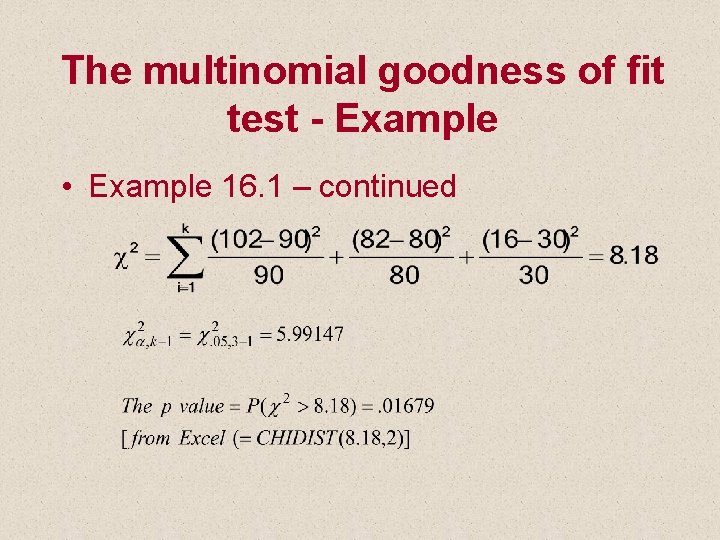
The multinomial goodness of fit test - Example • Example 16. 1 – continued

The multinomial goodness of fit test - Example • Example 16. 1 – continued c 2 with 2 degrees of freedom Conclusion: Since 8. 18 > 5. 99, there is sufficient evidence at 5% significance level to reject the null hypothesis. At least one of the probabilities pi is different. Thus, at least two market shares have changed. Alpha P value 5. 99 8. 18 Rejection region

Required conditions – the rule of five • The test statistic used to perform the test is only approximately Chi-squared distributed. • For the approximation to apply, the expected cell frequency has to be at least 5 for all the cells (npi ³ 5). • If the expected frequency in a cell is less than 5, combine it with other cells.

16. 3 Chi-squared Test of a Contingency Table • This test is used to test whether… – two nominal variables are related? – there are differences between two or more populations of a nominal variable • To accomplish the test objectives, we need to classify the data according to two different criteria.

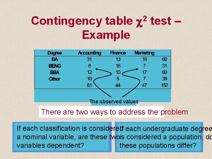
Contingency table c 2 test – Example • Example 16. 2 – In an effort to better predict the demand for courses offered by a certain MBA program, it was hypothesized that students’ academic background affect their choice of MBA major, thus, their courses selection. – A random sample of last year’s MBA students was selected. The following contingency table summarizes relevant data.

Contingency table c 2 test – Example The observed values There are two ways to address the problem If each classification is considered If each undergraduate degree a nominal variable, are these twois considered a population, do variables dependent? these populations differ?

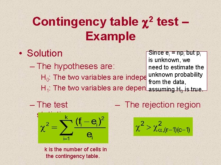
Contingency table c 2 test – Example • Solution – The hypotheses are: H 0: The two variables are H 1: The two variables are – The test statistic k is the number of cells in the contingency table. Since ei = npi but pi is unknown, we need to estimate the unknown probability independent from the data, dependent assuming H 0 is true. – The rejection region

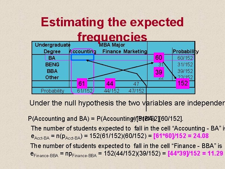
Estimating the expected frequencies Undergraduate MBA Major Degree Accounting Finance Marketing BA BENG BBA Other 61 44 47 Probability 61/152 44/152 47/152 60 60 31 39 39 22 Probability 60/152 31/152 39/152 22/152 152 Under the null hypothesis the two variables are independen P(Accounting and BA) = P(Accounting)*P(BA) = [61/152][60/152]. The number of students expected to fall in the cell “Accounting - BA” is e. Acct-BA = n(p. Acct-BA) = 152(61/152)(60/152) = [61*60]/152 = 24. 08 The number of students expected to fall in the cell “Finance - BBA” is e. Finance-BBA = np. Finance-BBA = 152(44/152)(39/152) = [44*39]/152 = 11. 29

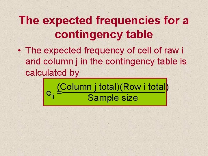
The expected frequencies for a contingency table • The expected frequency of cell of raw i and column j in the contingency table is calculated by (Column j total)(Row i total) eij = Sample size

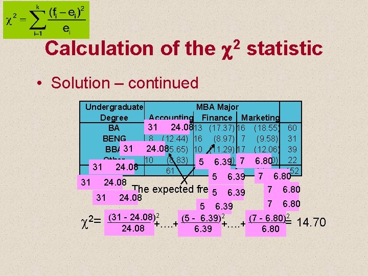
Calculation of the c 2 statistic • Solution – continued Undergraduate MBA Major Degree Accounting Finance Marketing 31 (24. 08) 24. 0813 (17. 37) 16 (18. 55) BA 31 BENG 8 (12. 44) 16 (8. 97) 7 (9. 58) 24. 08 BBA 31 12 (15. 65) 10 (11. 29) 17 (12. 06) Other 10 (8. 83) 55 (6. 39) (6. 80) 6. 39 77 6. 80 31 24. 08 61 44 47 31 24. 08 31 c 2= 5 6. 39 The expected frequency 5 6. 39 24. 08 7 60 31 39 22 152 6. 80 7 6. 80 5 6. 39 (31 - 24. 08)2 (5 - 6. 39)2 (7 - 6. 80)2 = 14. 70 24. 08 +…. + 6. 39 +…. + 6. 80

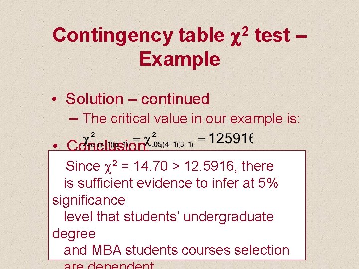
Contingency table c 2 test – Example • Solution – continued – The critical value in our example is: • Conclusion: Since c 2 = 14. 70 > 12. 5916, there is sufficient evidence to infer at 5% significance level that students’ undergraduate degree and MBA students courses selection

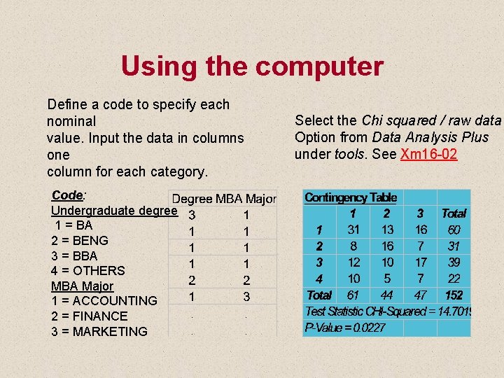
Using the computer Define a code to specify each nominal value. Input the data in columns one column for each category. Code: Undergraduate degree 1 = BA 2 = BENG 3 = BBA 4 = OTHERS MBA Major 1 = ACCOUNTING 2 = FINANCE 3 = MARKETING Select the Chi squared / raw data Option from Data Analysis Plus under tools. See Xm 16 -02

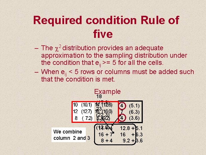
Required condition Rule of five – The c 2 distribution provides an adequate approximation to the sampling distribution under the condition that eij >= 5 for all the cells. – When eij < 5 rows or columns must be added such that the condition is met. Example We combine column 2 and 3 18 (17. 9) 23 (22. 3) 12 (12. 8) 14 + 4 16 + 7 8+4 4 7 4 (5. 1) (6. 3) (3. 6) 12. 8 + 5. 1 16 + 6. 3 9. 2 + 3. 6

16. 5 Chi-Squared test for Normality • The goodness of fit Chi-squared test can be used to determined if data were drawn from any distribution. • The general procedure: – Hypothesize on the parameter values of the distribution we test (i. e. m = m 0, s = s 0 for the normal distribution). – For the variable tested X specify disjoint ranges that cover all its possible values. – Build a Chi squared statistic that (aggregately) compares the expected frequency under H 0 and the actual frequency of observations that fall in each range.

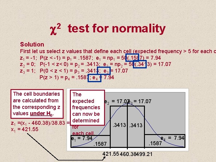
15. 5 Chi-Squared test for Normality • Testing for normality in Example 12. 1 For a sample size of n=50 (see Xm 12 -01) , the sample mean was 460. 38 with standard error of 38. 83. Can we infer from the data provided that this sample was drawn from a normal distribution with m = 460. 38 and s = 38. 83? Use 5% significance level.

c 2 test for normality Solution First let us select z values that define each cell (expected frequency > 5 for each c z 1 = -1; P(z < -1) = p 1 =. 1587; e 1 = np 1 = 50(. 1587) = 7. 94 z 2 = 0; P(-1 < z< 0) = p 2 =. 3413; e 2 = np 2 = 50(. 3413) = 17. 07 z 3 = 1; P(0 < z < 1) = p 3 =. 3413; e 3 = 17. 07 P(z > 1) = p 4 =. 1587; e 4 = 7. 94 The cell boundaries are calculated from the corresponding z values under H 0. The expected e 2 = 17. 07 e 3 = 17. 07 frequencies can now be determined z 1 =(x 1 - 460. 38)/38. 83 = -1; . 3413 for x 1 = 421. 55 each cell. e 4 = 7. 94 e 1 = 7. 94. 1587 421. 55 460. 38499. 21

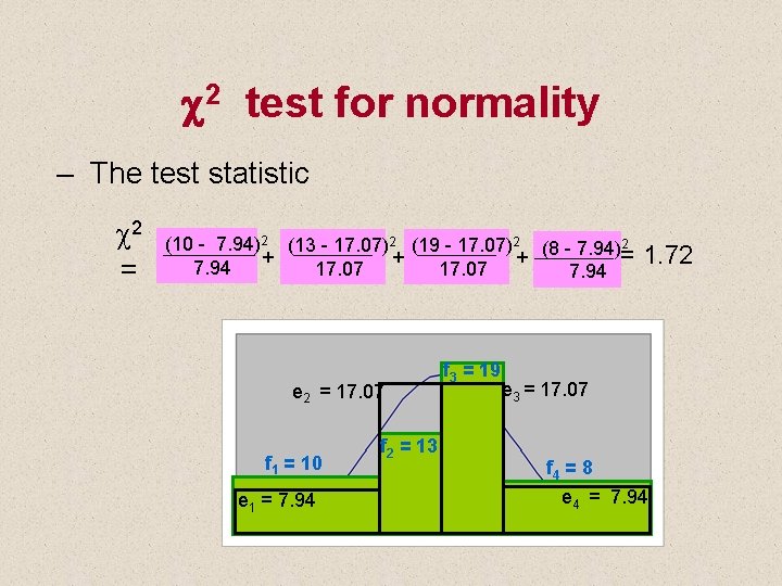
c 2 test for normality – The test statistic c 2 = (10 - 7. 94)2 (13 - 17. 07)2 (19 - 17. 07)2 (8 - 7. 94)2 = + + + 7. 94 17. 07 7. 94 e 2 = 17. 07 f 1 = 10 e 1 = 7. 94 f 2 = 13 f 3 = 19 1. 72 e 3 = 17. 07 f 4 = 8 e 4 = 7. 94

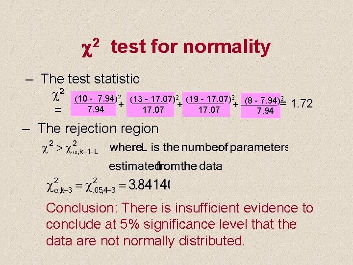
c 2 test for normality – The test statistic c 2 (10 - 7. 94)2 (13 - 17. 07)2 (19 - 17. 07)2 + + + 7. 94 17. 07 = – The rejection region 2 (8 - 7. 94)= 7. 94 1. 72 Conclusion: There is insufficient evidence to conclude at 5% significance level that the data are not normally distributed.