Chapter 16 17 Analysis of Variance Correlation and

Chapter 16 & 17 Analysis of Variance Correlation and Regression Analysis Copyright © 2010 Pearson Education, Inc. 16 -1

Chapter Outline 1) Overview 2) Relationship Among Techniques 3) One-Way Analysis of Variance 4) Statistics Associated with One-Way Analysis of Variance 5) Conducting One-Way Analysis of Variance i. Identification of Dependent & Independent Variables ii. Decomposition of the Total Variation iii. Measurement of Effects iv. Significance Testing v. Interpretation of Results Copyright © 2010 Pearson Education, Inc. 16 -2

Chapter Outline 1) 2) 3) 4) 5) Overview Product-Moment Correlation Regression Analysis Bivariate Regression Statistics Associated with Bivariate Regression Analysis 6) Conducting Bivariate Regression Analysis i. Scatter Diagram ii. Bivariate Regression Model 7) Multiple Regression Copyright © 2010 Pearson Education, Inc. 16 -3

Relationship Among Techniques • Analysis of variance (ANOVA) is used as a test of means for two or more populations. The null hypothesis, typically, is that all means are equal. • Analysis of variance must have a dependent variable that is metric (measured using an interval or ratio scale). • There must also be one or more independent variables that are all categorical (nonmetric). Categorical independent variables are also called factors. Copyright © 2010 Pearson Education, Inc. 16 -4

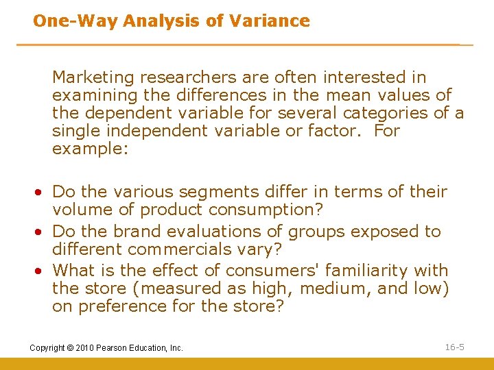
One-Way Analysis of Variance Marketing researchers are often interested in examining the differences in the mean values of the dependent variable for several categories of a single independent variable or factor. For example: • Do the various segments differ in terms of their volume of product consumption? • Do the brand evaluations of groups exposed to different commercials vary? • What is the effect of consumers' familiarity with the store (measured as high, medium, and low) on preference for the store? Copyright © 2010 Pearson Education, Inc. 16 -5

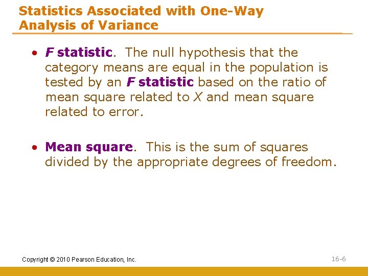
Statistics Associated with One-Way Analysis of Variance • F statistic. The null hypothesis that the category means are equal in the population is tested by an F statistic based on the ratio of mean square related to X and mean square related to error. • Mean square. This is the sum of squares divided by the appropriate degrees of freedom. Copyright © 2010 Pearson Education, Inc. 16 -6

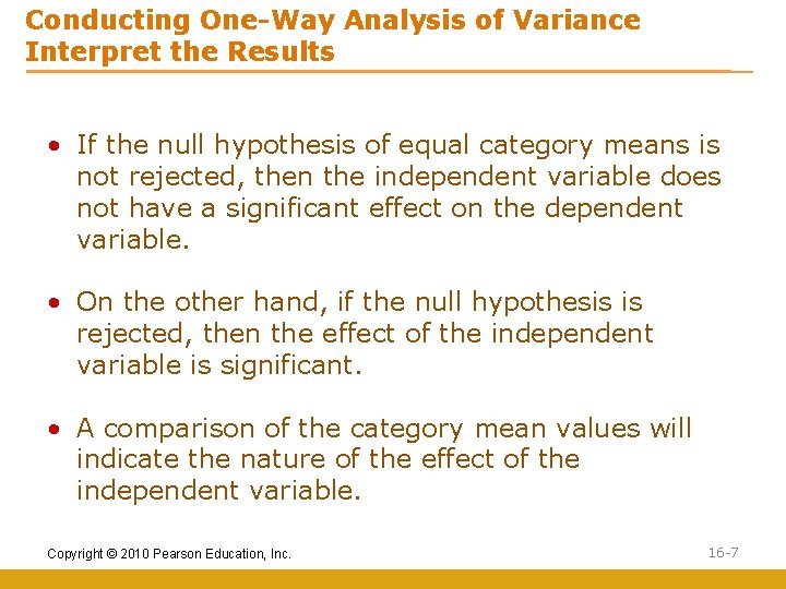
Conducting One-Way Analysis of Variance Interpret the Results • If the null hypothesis of equal category means is not rejected, then the independent variable does not have a significant effect on the dependent variable. • On the other hand, if the null hypothesis is rejected, then the effect of the independent variable is significant. • A comparison of the category mean values will indicate the nature of the effect of the independent variable. Copyright © 2010 Pearson Education, Inc. 16 -7

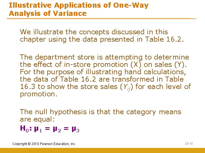
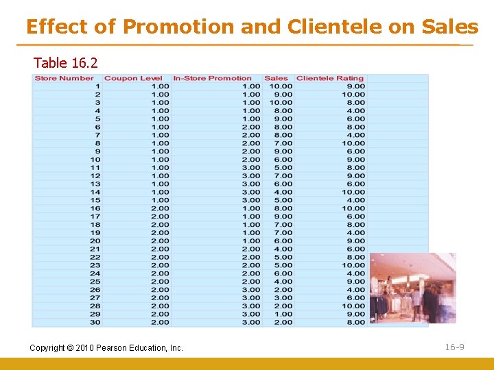
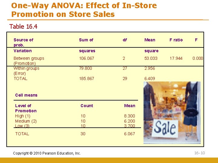
Illustrative Applications of One-Way Analysis of Variance We illustrate the concepts discussed in this chapter using the data presented in Table 16. 2. The department store is attempting to determine the effect of in-store promotion (X) on sales (Y). For the purpose of illustrating hand calculations, the data of Table 16. 2 are transformed in Table 16. 3 to show the store sales (Yij) for each level of promotion. The null hypothesis is that the category means are equal: H 0 : µ 1 = µ 2 = µ 3 Copyright © 2010 Pearson Education, Inc. 16 -8

Effect of Promotion and Clientele on Sales Table 16. 2 Copyright © 2010 Pearson Education, Inc. 16 -9

One-Way ANOVA: Effect of In-Store Promotion on Store Sales Table 16. 4 Source of prob. Variation Sum of df Between groups (Promotion) Within groups (Error) TOTAL 106. 067 2 53. 033 79. 800 27 2. 956 185. 867 29 6. 409 squares Mean F ratio F square 17. 944 0. 000 Cell means Level of Promotion High (1) Medium (2) Low (3) Count Mean 10 10 10 8. 300 6. 200 3. 700 TOTAL 30 6. 067 Copyright © 2010 Pearson Education, Inc. 16 -10

Multivariate Analysis of Variance • Multivariate analysis of variance (MANOVA) is similar to analysis of variance (ANOVA), except that instead of one metric dependent variable, we have two or more. • In MANOVA, the null hypothesis is that the vectors of means on multiple dependent variables are equal across groups. • Multivariate analysis of variance is appropriate when there are two or more dependent variables that are correlated. Copyright © 2010 Pearson Education, Inc. 16 -11

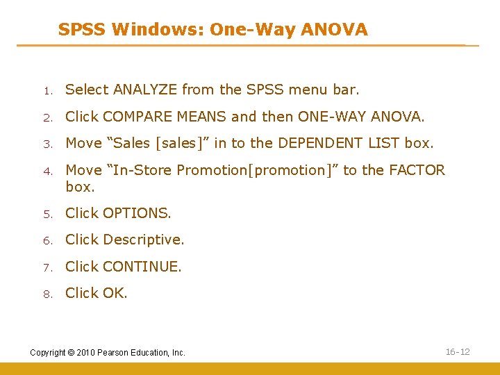
SPSS Windows: One-Way ANOVA 1. Select ANALYZE from the SPSS menu bar. 2. Click COMPARE MEANS and then ONE-WAY ANOVA. 3. Move “Sales [sales]” in to the DEPENDENT LIST box. 4. Move “In-Store Promotion[promotion]” to the FACTOR box. 5. Click OPTIONS. 6. Click Descriptive. 7. Click CONTINUE. 8. Click OK. Copyright © 2010 Pearson Education, Inc. 16 -12

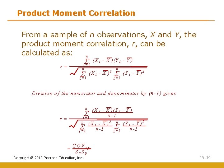
Correlation • The product moment correlation, r, summarizes the strength of association between two metric (interval or ratio scaled) variables, say X and Y. • It is an index used to determine whether a linear or straightline relationship exists between X and Y. • As it was originally proposed by Karl Pearson, it is also known as the Pearson correlation coefficient. It is also referred to as simple correlation, bivariate correlation, or merely the correlation coefficient. Copyright © 2010 Pearson Education, Inc. 16 -13

Product Moment Correlation From a sample of n observations, X and Y, the product moment correlation, r, can be calculated as: n r= S i =1 n S i =1 (X i - X )(Y i - Y ) (X i - X ) 2 n S i =1 (Y i - Y )2 D iv is io n o f th e n u m erato r an d d en o m in ato r b y ( n - 1 ) g iv es n S i =1 r= n S i =1 = ( X i - X )( Y i - Y ) n -1 (X i - X )2 n -1 n S i =1 (Y i - Y )2 n -1 C OV x y Sx. Sy Copyright © 2010 Pearson Education, Inc. 16 -14

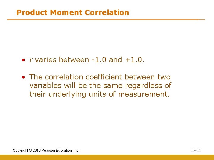
Product Moment Correlation • r varies between -1. 0 and +1. 0. • The correlation coefficient between two variables will be the same regardless of their underlying units of measurement. Copyright © 2010 Pearson Education, Inc. 16 -15

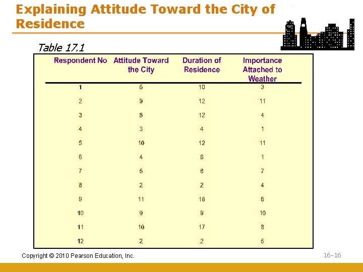
Explaining Attitude Toward the City of Residence Table 17. 1 Copyright © 2010 Pearson Education, Inc. 16 -16

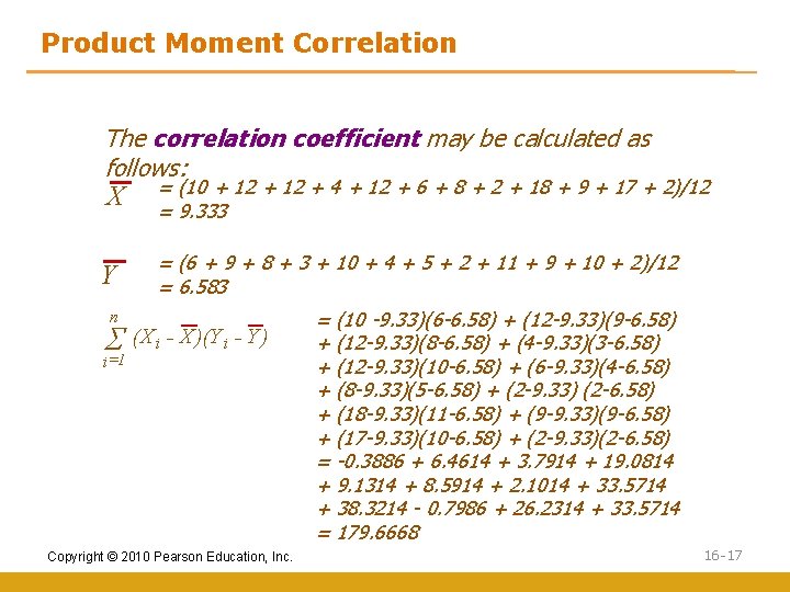
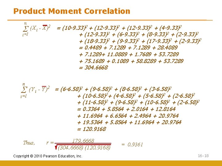
Product Moment Correlation The correlation coefficient may be calculated as follows: X Y = (10 + 12 + 4 + 12 + 6 + 8 + 2 + 18 + 9 + 17 + 2)/12 = 9. 333 = (6 + 9 + 8 + 3 + 10 + 4 + 5 + 2 + 11 + 9 + 10 + 2)/12 = 6. 583 n S=1 (X i - X )(Y i - Y ) i Copyright © 2010 Pearson Education, Inc. = (10 -9. 33)(6 -6. 58) + (12 -9. 33)(9 -6. 58) + (12 -9. 33)(8 -6. 58) + (4 -9. 33)(3 -6. 58) + (12 -9. 33)(10 -6. 58) + (6 -9. 33)(4 -6. 58) + (8 -9. 33)(5 -6. 58) + (2 -9. 33) (2 -6. 58) + (18 -9. 33)(11 -6. 58) + (9 -9. 33)(9 -6. 58) + (17 -9. 33)(10 -6. 58) + (2 -9. 33)(2 -6. 58) = -0. 3886 + 6. 4614 + 3. 7914 + 19. 0814 + 9. 1314 + 8. 5914 + 2. 1014 + 33. 5714 + 38. 3214 - 0. 7986 + 26. 2314 + 33. 5714 = 179. 6668 16 -17

Product Moment Correlation n S=1 (X i - X )2 i n S i =1 = (10 -9. 33)2 + (12 -9. 33)2 + (4 -9. 33)2 + (12 -9. 33)2 + (6 -9. 33)2 + (8 -9. 33)2 + (2 -9. 33)2 + (18 -9. 33)2 + (9 -9. 33)2 + (17 -9. 33)2 + (2 -9. 33)2 = 0. 4489 + 7. 1289 + 28. 4089 + 7. 1289+ 11. 0889 + 1. 7689 + 53. 7289 + 75. 1689 + 0. 1089 + 58. 8289 + 53. 7289 = 304. 6668 (Y i - Y )2 = (6 -6. 58)2 + (9 -6. 58)2 + (8 -6. 58)2 + (3 -6. 58)2 + (10 -6. 58)2+ (4 -6. 58)2 + (5 -6. 58)2 + (2 -6. 58)2 + (11 -6. 58)2 + (9 -6. 58)2 + (10 -6. 58)2 + (2 -6. 58)2 = 0. 3364 + 5. 8564 + 2. 0164 + 12. 8164 + 11. 6964 + 6. 6564 + 2. 4964 + 20. 9764 + 19. 5364 + 5. 8564 + 11. 6964 + 20. 9764 = 120. 9168 Thus, r= 179. 6668 (304. 6668) (120. 9168) Copyright © 2010 Pearson Education, Inc. = 0. 9361 16 -18

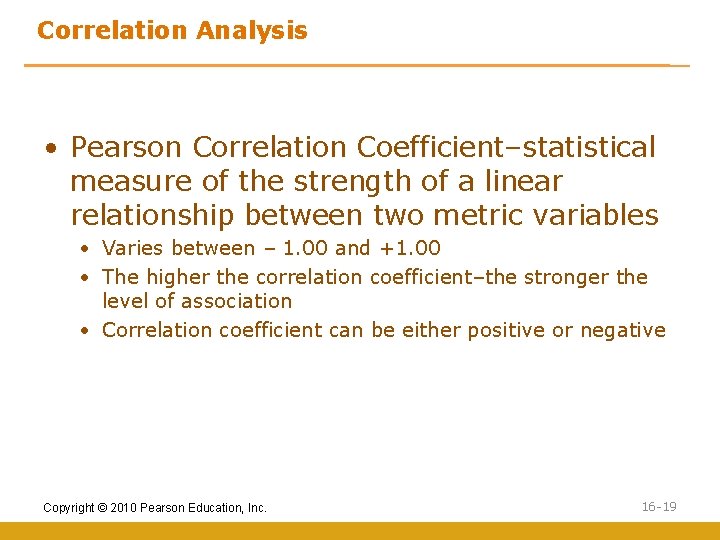
Correlation Analysis • Pearson Correlation Coefficient–statistical measure of the strength of a linear relationship between two metric variables • Varies between – 1. 00 and +1. 00 • The higher the correlation coefficient–the stronger the level of association • Correlation coefficient can be either positive or negative Copyright © 2010 Pearson Education, Inc. 16 -19

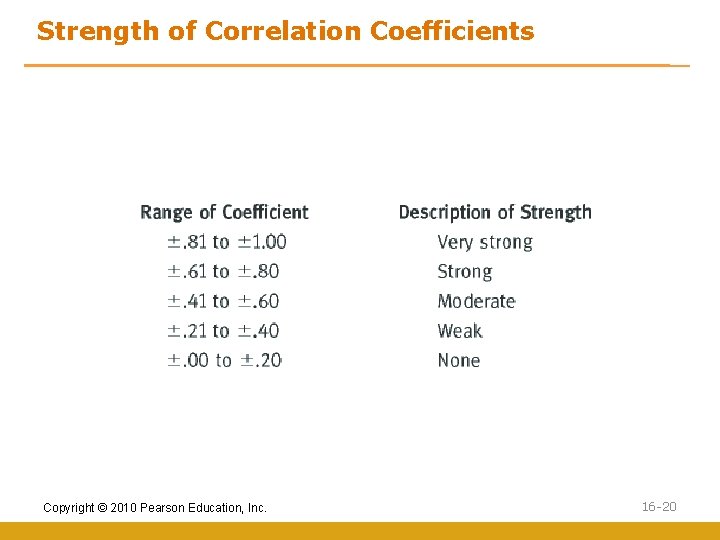
Strength of Correlation Coefficients Copyright © 2010 Pearson Education, Inc. 16 -20

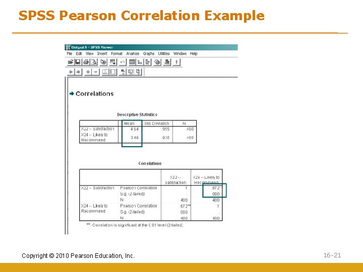
SPSS Pearson Correlation Example Copyright © 2010 Pearson Education, Inc. 16 -21

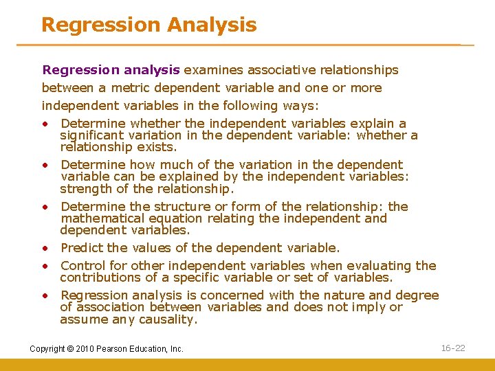
Regression Analysis Regression analysis examines associative relationships between a metric dependent variable and one or more independent variables in the following ways: • Determine whether the independent variables explain a significant variation in the dependent variable: whether a relationship exists. • Determine how much of the variation in the dependent variable can be explained by the independent variables: strength of the relationship. • Determine the structure or form of the relationship: the mathematical equation relating the independent and dependent variables. • Predict the values of the dependent variable. • Control for other independent variables when evaluating the contributions of a specific variable or set of variables. • Regression analysis is concerned with the nature and degree of association between variables and does not imply or assume any causality. Copyright © 2010 Pearson Education, Inc. 16 -22

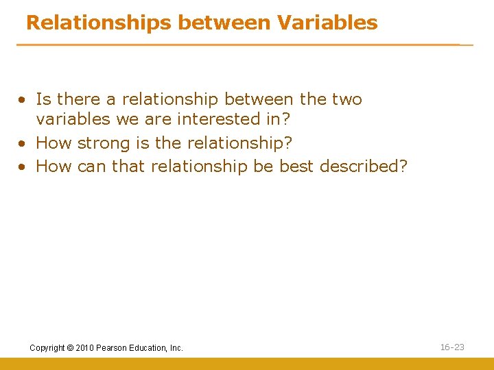
Relationships between Variables • Is there a relationship between the two variables we are interested in? • How strong is the relationship? • How can that relationship be best described? Copyright © 2010 Pearson Education, Inc. 16 -23

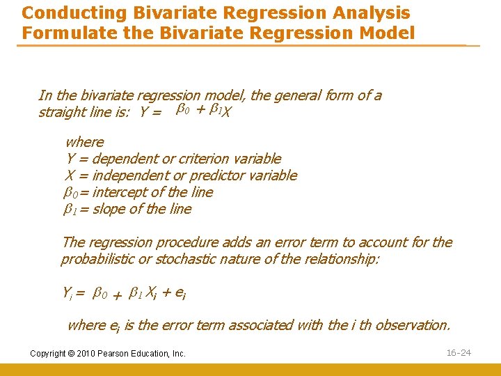
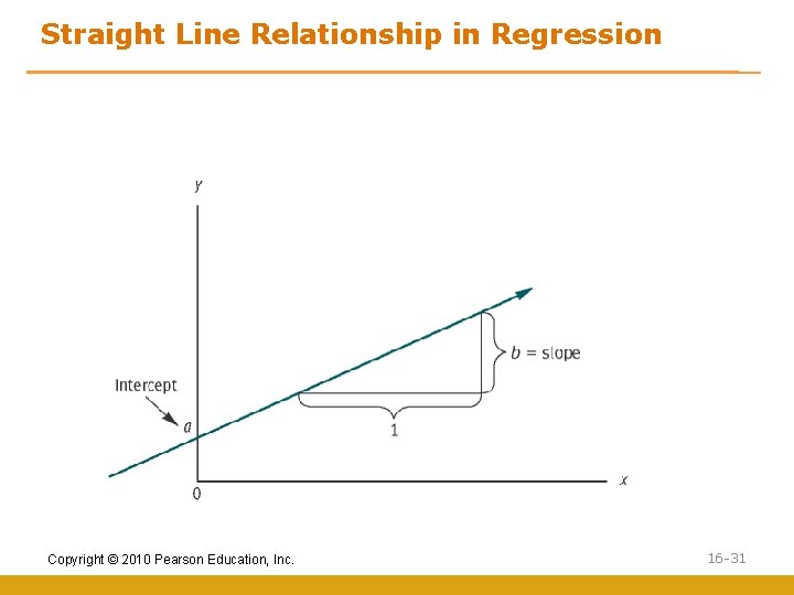
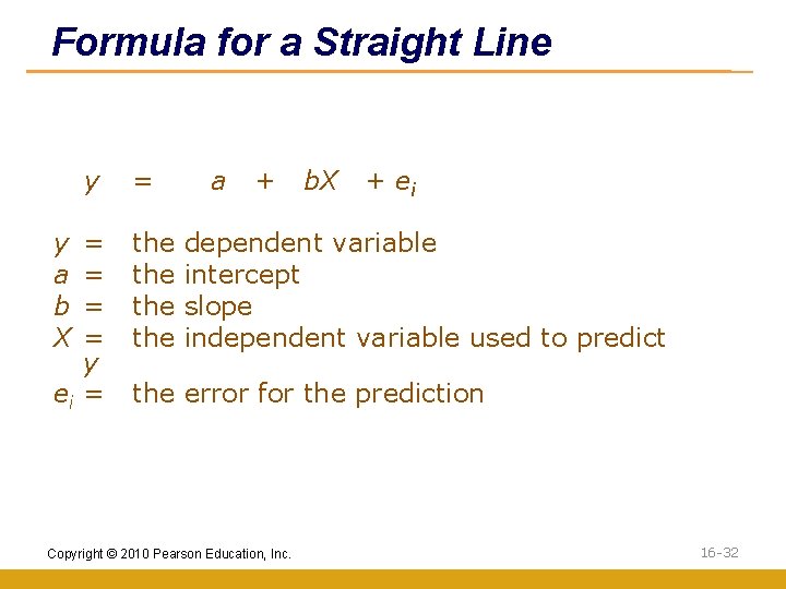
Conducting Bivariate Regression Analysis Formulate the Bivariate Regression Model In the bivariate regression model, the general form of a straight line is: Y = b 0 + b 1 X where Y = dependent or criterion variable X = independent or predictor variable b 0= intercept of the line b 1= slope of the line The regression procedure adds an error term to account for the probabilistic or stochastic nature of the relationship: Yi = b 0 + b 1 X i + e i where ei is the error term associated with the i th observation. Copyright © 2010 Pearson Education, Inc. 16 -24

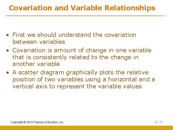
Covariation and Variable Relationships • First we should understand the covariation between variables • Covariation is amount of change in one variable that is consistently related to the change in another variable • A scatter diagram graphically plots the relative position of two variables using a horizontal and a vertical axis to represent the variable values Copyright © 2010 Pearson Education, Inc. 16 -25

Plot of Attitude with Duration Attitude Fig. 17. 3 9 6 3 2. 25 4. 5 6. 75 9 11. 25 13. 5 15. 75 18 Duration of Residence Copyright © 2010 Pearson Education, Inc. 16 -26

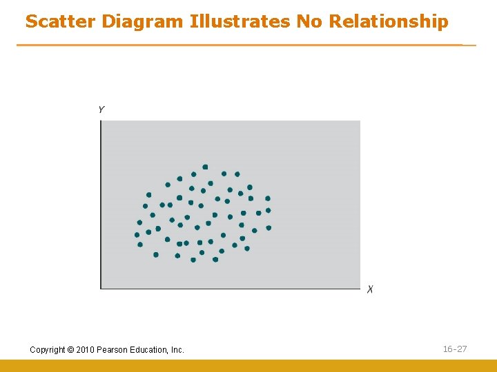
Scatter Diagram Illustrates No Relationship Copyright © 2010 Pearson Education, Inc. 16 -27

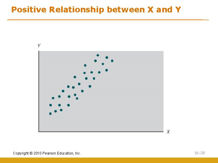
Positive Relationship between X and Y Copyright © 2010 Pearson Education, Inc. 16 -28

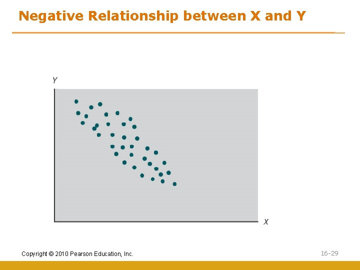
Negative Relationship between X and Y Copyright © 2010 Pearson Education, Inc. 16 -29

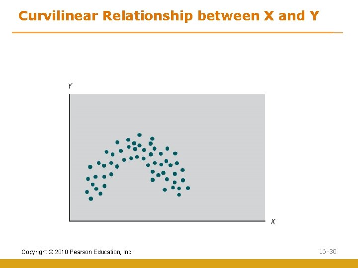
Curvilinear Relationship between X and Y Copyright © 2010 Pearson Education, Inc. 16 -30

Straight Line Relationship in Regression Copyright © 2010 Pearson Education, Inc. 16 -31

Formula for a Straight Line y y a b X = = y ei = = the the a + b. X + ei dependent variable intercept slope independent variable used to predict the error for the prediction Copyright © 2010 Pearson Education, Inc. 16 -32

Ordinary Least Squares (OLS) OLS is a statistical procedure that estimates regression equation coefficients which produce the lowest sum of squared differences between the actual and predicted values of the dependent variable Copyright © 2010 Pearson Education, Inc. 16 -33

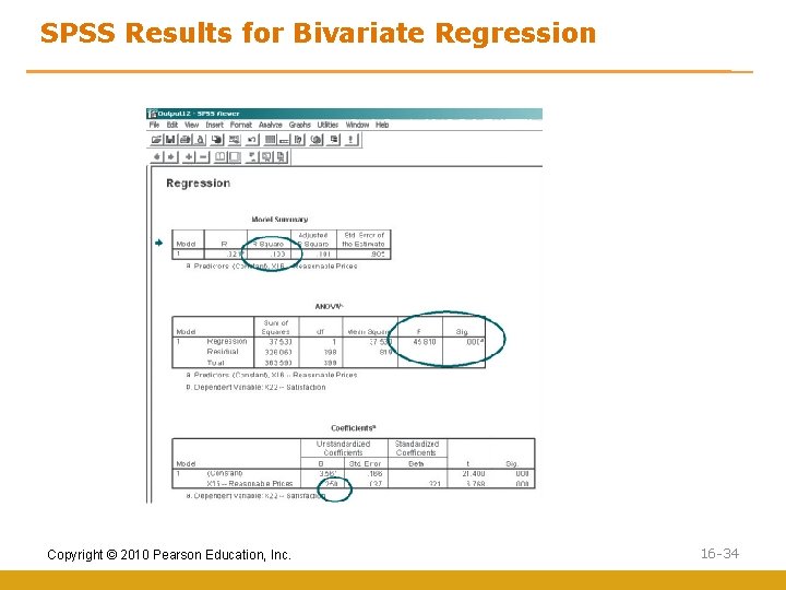
SPSS Results for Bivariate Regression Copyright © 2010 Pearson Education, Inc. 16 -34

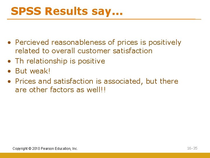
SPSS Results say. . . • Percieved reasonableness of prices is positively related to overall customer satisfaction • Th relationship is positive • But weak! • Prices and satisfaction is associated, but there are other factors as well!! Copyright © 2010 Pearson Education, Inc. 16 -35

Multiple Regression Analysis Multiple regression analysis is a statistical technique which analyzes the linear relationship between a dependent variable and multiple independent variables by estimating coefficients for the equation for a straight line Copyright © 2010 Pearson Education, Inc. 16 -36

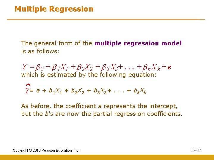
Multiple Regression The general form of the multiple regression model is as follows: Y = b 0 + b 1 X 1 + b 2 X 2 + b 3 X 3+. . . + b k X k + e which is estimated by the following equation: Y= a + b 1 X 1 + b 2 X 2 + b 3 X 3+. . . + bk. Xk As before, the coefficient a represents the intercept, but the b's are now the partial regression coefficients. Copyright © 2010 Pearson Education, Inc. 16 -37

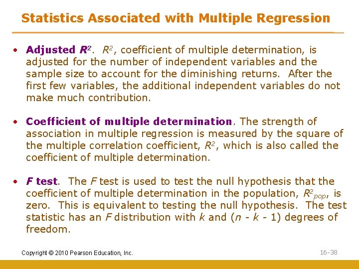
Statistics Associated with Multiple Regression • Adjusted R 2, coefficient of multiple determination, is adjusted for the number of independent variables and the sample size to account for the diminishing returns. After the first few variables, the additional independent variables do not make much contribution. • Coefficient of multiple determination. The strength of association in multiple regression is measured by the square of the multiple correlation coefficient, R 2, which is also called the coefficient of multiple determination. • F test. The F test is used to test the null hypothesis that the coefficient of multiple determination in the population, R 2 pop, is zero. This is equivalent to testing the null hypothesis. The test statistic has an F distribution with k and (n - k - 1) degrees of freedom. Copyright © 2010 Pearson Education, Inc. 16 -38

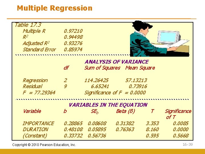
Multiple Regression Table 17. 3 Multiple R R 2 Adjusted R 2 Standard Error 0. 97210 0. 94498 0. 93276 0. 85974 df Regression Residual F = 77. 29364 2 9 ANALYSIS OF VARIANCE Sum of Squares Mean Square 114. 26425 57. 13213 6. 65241 0. 73916 Significance of F = 0. 0000 Variable VARIABLES IN THE EQUATION b SEb Beta (ß) T IMPORTANCE DURATION (Constant) 0. 28865 0. 08608 0. 48108 0. 05895 0. 33732 0. 56736 Copyright © 2010 Pearson Education, Inc. 0. 31382 0. 76363 3. 353 8. 160 0. 595 Significance of T 0. 0085 0. 0000 0. 5668 16 -39

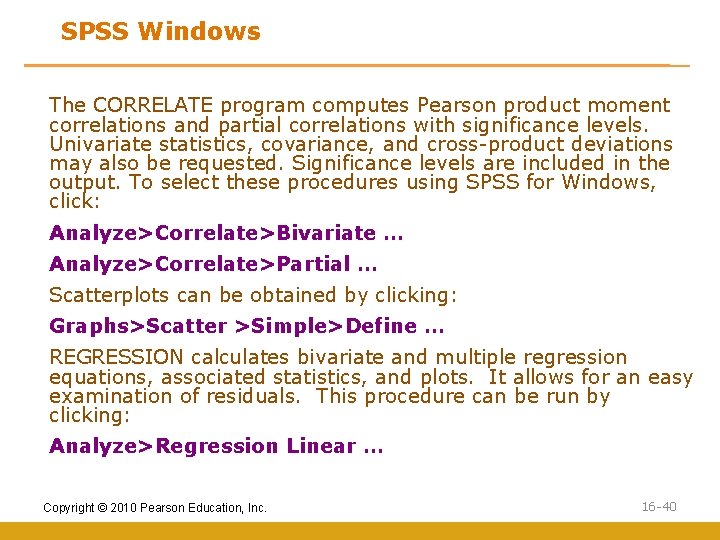
SPSS Windows The CORRELATE program computes Pearson product moment correlations and partial correlations with significance levels. Univariate statistics, covariance, and cross-product deviations may also be requested. Significance levels are included in the output. To select these procedures using SPSS for Windows, click: Analyze>Correlate>Bivariate … Analyze>Correlate>Partial … Scatterplots can be obtained by clicking: Graphs>Scatter >Simple>Define … REGRESSION calculates bivariate and multiple regression equations, associated statistics, and plots. It allows for an easy examination of residuals. This procedure can be run by clicking: Analyze>Regression Linear … Copyright © 2010 Pearson Education, Inc. 16 -40

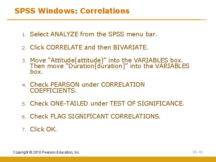
SPSS Windows: Correlations 1. Select ANALYZE from the SPSS menu bar. 2. Click CORRELATE and then BIVARIATE. 3. Move “Attitude[attitude]” into the VARIABLES box. Then move “Duration[duration]” into the VARIABLES box. 4. Check PEARSON under CORRELATION COEFFICIENTS. 5. Check ONE-TAILED under TEST OF SIGNIFICANCE. 6. Check FLAG SIGNIFICANT CORRELATIONS. 7. Click OK. Copyright © 2010 Pearson Education, Inc. 16 -41

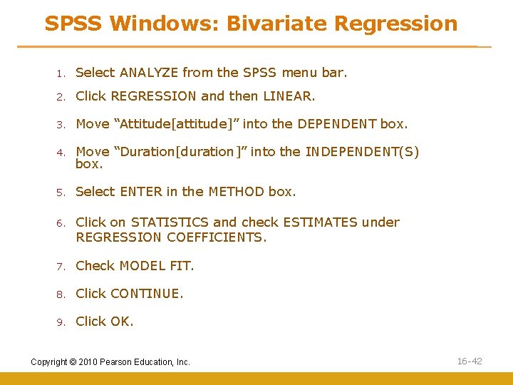
SPSS Windows: Bivariate Regression 1. Select ANALYZE from the SPSS menu bar. 2. Click REGRESSION and then LINEAR. 3. Move “Attitude[attitude]” into the DEPENDENT box. 4. Move “Duration[duration]” into the INDEPENDENT(S) box. 5. Select ENTER in the METHOD box. 6. Click on STATISTICS and check ESTIMATES under REGRESSION COEFFICIENTS. 7. Check MODEL FIT. 8. Click CONTINUE. 9. Click OK. Copyright © 2010 Pearson Education, Inc. 16 -42

All rights reserved. No part of this publication may be reproduced, stored in a retrieval system, or transmitted, in any form or by any means, electronic, mechanical, photocopying, recording, or otherwise, without the prior written permission of the publisher. Printed in the United States of America. Copyright © 2010 Pearson Education, Inc. 16 -43