Chapter 15 TwoFactor Analysis of Variance 1 TwoFactor

Chapter 15: Two-Factor Analysis of Variance 1

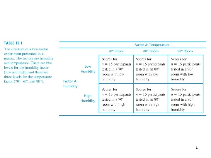
Two-Factor Designs • In the context of ANOVA, an independent variable (or a quasi-independent variable) is called a factor, and research studies with two factors are called factorial designs or simply two-factor designs. • The two factors are identified as A and B, and the structure of a two-factor design can be represented as a matrix with the levels of factor A determining the rows and the levels of factor B determining the columns. 2

3

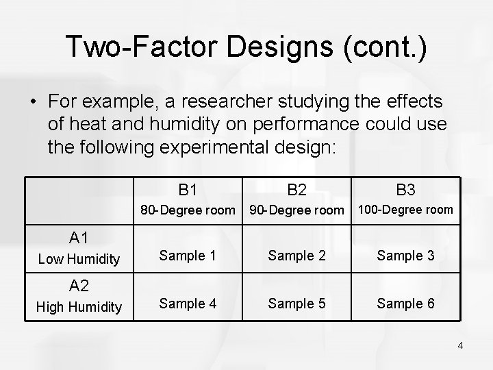
Two-Factor Designs (cont. ) • For example, a researcher studying the effects of heat and humidity on performance could use the following experimental design: B 1 B 2 B 3 80 -Degree room 90 -Degree room 100 -Degree room Sample 1 Sample 2 Sample 3 Sample 4 Sample 5 Sample 6 A 1 Low Humidity A 2 High Humidity 4

5

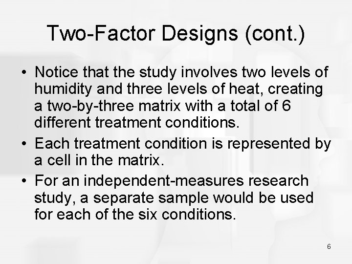
Two-Factor Designs (cont. ) • Notice that the study involves two levels of humidity and three levels of heat, creating a two-by-three matrix with a total of 6 different treatment conditions. • Each treatment condition is represented by a cell in the matrix. • For an independent-measures research study, a separate sample would be used for each of the six conditions. 6

7

Main Effects and Interactions • The goal for the two-factor ANOVA is to determine whether the mean differences that are observed for the sample data are sufficiently large to conclude that they are significant differences and not simply the result of sampling error. • For the example we are considering, the goal is to determine whether different levels of heat and humidity produce significant differences in performance. 8

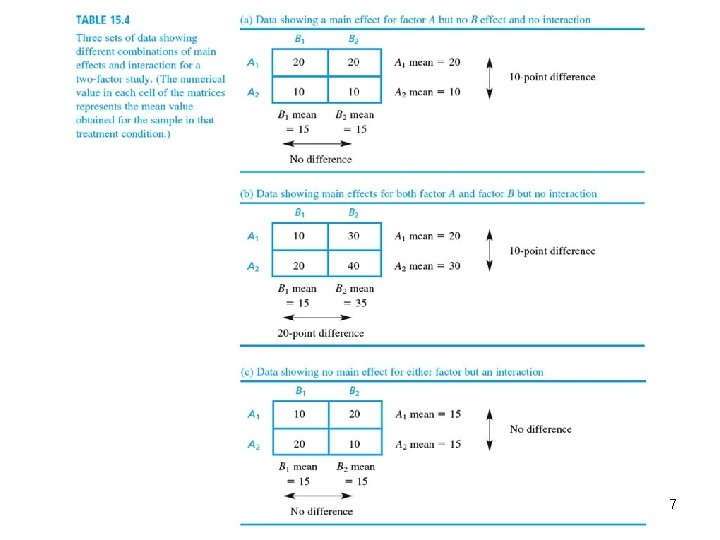
Main Effects and Interactions (cont. ) To evaluate the sample mean differences, a twofactor ANOVA conducts three separate and independent hypothesis tests. The three tests evaluate: 1. The Main Effect for Factor A The mean differences between the levels of factor A are obtained by computing the overall mean for each row in the matrix. In this example, the main effect of factor A would compare the overall mean performance with high humidity versus the overall mean performance with low humidity. 9

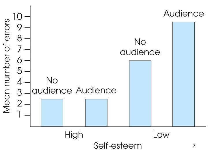
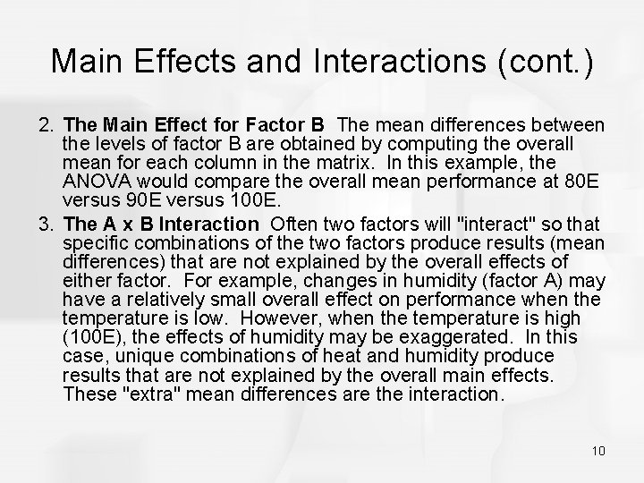
Main Effects and Interactions (cont. ) 2. The Main Effect for Factor B The mean differences between the levels of factor B are obtained by computing the overall mean for each column in the matrix. In this example, the ANOVA would compare the overall mean performance at 80 E versus 90 E versus 100 E. 3. The A x B Interaction Often two factors will "interact" so that specific combinations of the two factors produce results (mean differences) that are not explained by the overall effects of either factor. For example, changes in humidity (factor A) may have a relatively small overall effect on performance when the temperature is low. However, when the temperature is high (100 E), the effects of humidity may be exaggerated. In this case, unique combinations of heat and humidity produce results that are not explained by the overall main effects. These "extra" mean differences are the interaction. 10

11

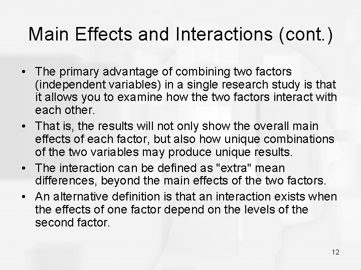
Main Effects and Interactions (cont. ) • The primary advantage of combining two factors (independent variables) in a single research study is that it allows you to examine how the two factors interact with each other. • That is, the results will not only show the overall main effects of each factor, but also how unique combinations of the two variables may produce unique results. • The interaction can be defined as "extra" mean differences, beyond the main effects of the two factors. • An alternative definition is that an interaction exists when the effects of one factor depend on the levels of the second factor. 12

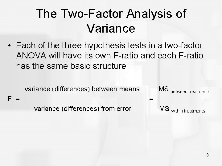
The Two-Factor Analysis of Variance • Each of the three hypothesis tests in a two-factor ANOVA will have its own F-ratio and each F-ratio has the same basic structure variance (differences) between means MS between treatments F = ───────────── = ───── variance (differences) from error MS within treatments 13

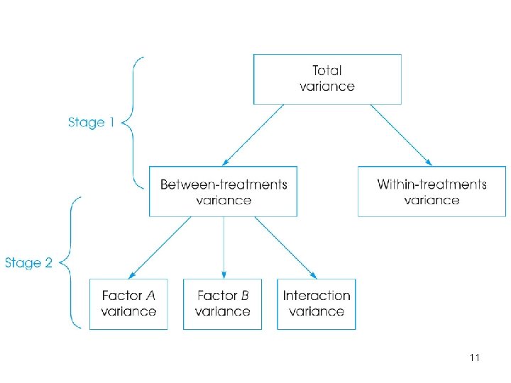
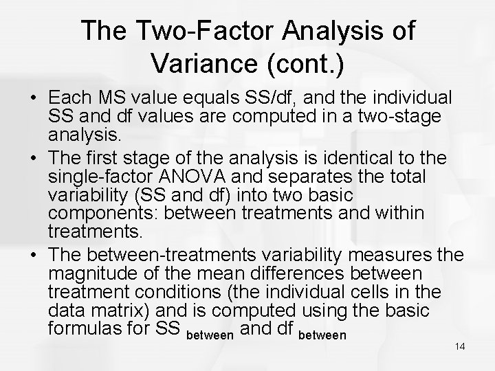
The Two-Factor Analysis of Variance (cont. ) • Each MS value equals SS/df, and the individual SS and df values are computed in a two-stage analysis. • The first stage of the analysis is identical to the single-factor ANOVA and separates the total variability (SS and df) into two basic components: between treatments and within treatments. • The between-treatments variability measures the magnitude of the mean differences between treatment conditions (the individual cells in the data matrix) and is computed using the basic formulas for SS between and df between 14

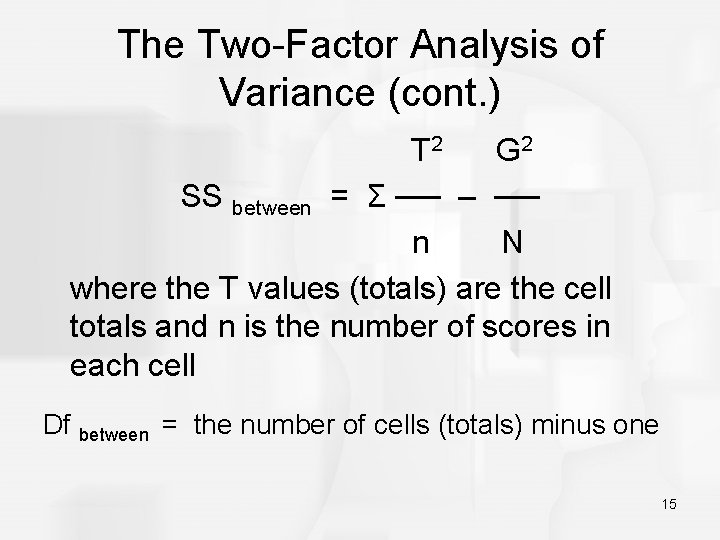
The Two-Factor Analysis of Variance (cont. ) T 2 G 2 SS between = Σ ── – ── n N where the T values (totals) are the cell totals and n is the number of scores in each cell Df between = the number of cells (totals) minus one 15

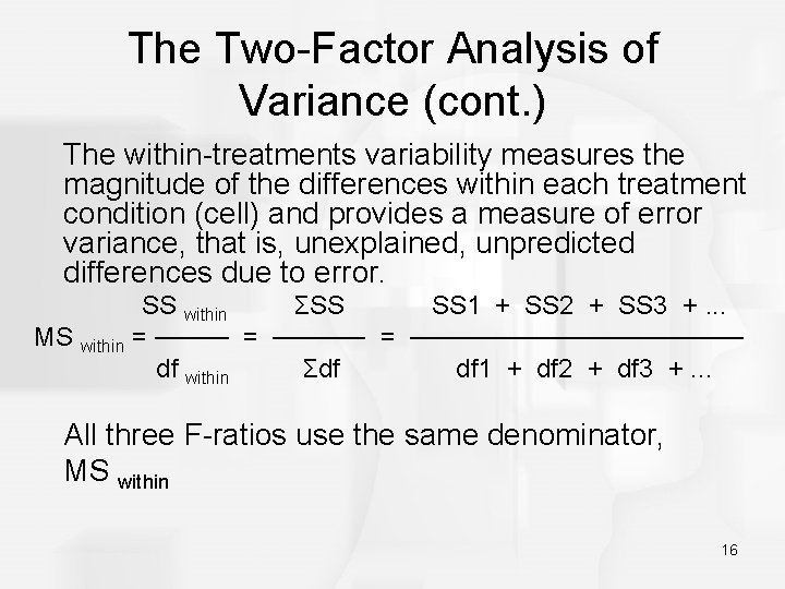
The Two-Factor Analysis of Variance (cont. ) The within-treatments variability measures the magnitude of the differences within each treatment condition (cell) and provides a measure of error variance, that is, unexplained, unpredicted differences due to error. SS within ΣSS SS 1 + SS 2 + SS 3 +. . . MS within = ───────── df within Σdf df 1 + df 2 + df 3 +. . . All three F-ratios use the same denominator, MS within 16

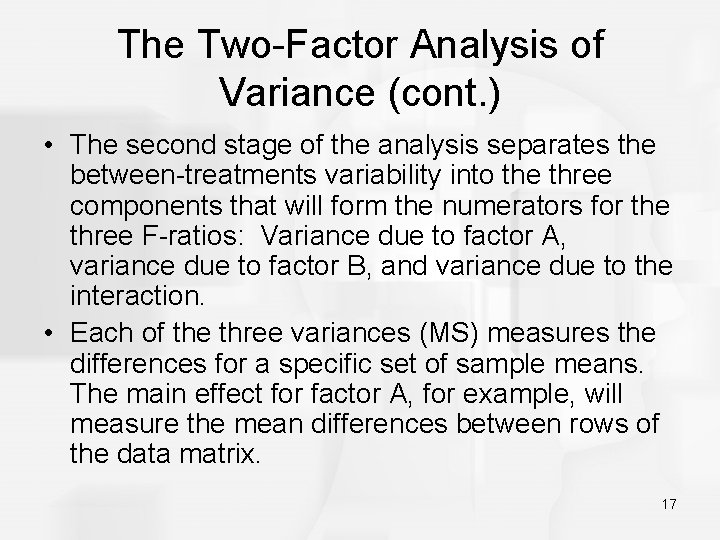
The Two-Factor Analysis of Variance (cont. ) • The second stage of the analysis separates the between-treatments variability into the three components that will form the numerators for the three F-ratios: Variance due to factor A, variance due to factor B, and variance due to the interaction. • Each of the three variances (MS) measures the differences for a specific set of sample means. The main effect for factor A, for example, will measure the mean differences between rows of the data matrix. 17

The Two-Factor Analysis of Variance (cont. ) • The actual formulas for each SS and df are based on the sample totals (rather than the means) and all have the same structure: 18

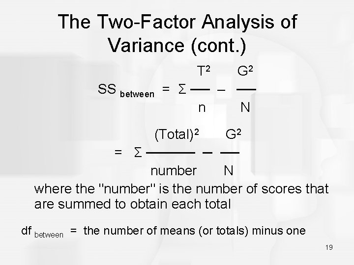
The Two-Factor Analysis of Variance (cont. ) SS between T 2 G 2 = Σ ── – ── n N (Total)2 G 2 = Σ ───── ─ ── number N where the "number" is the number of scores that are summed to obtain each total df between = the number of means (or totals) minus one 19

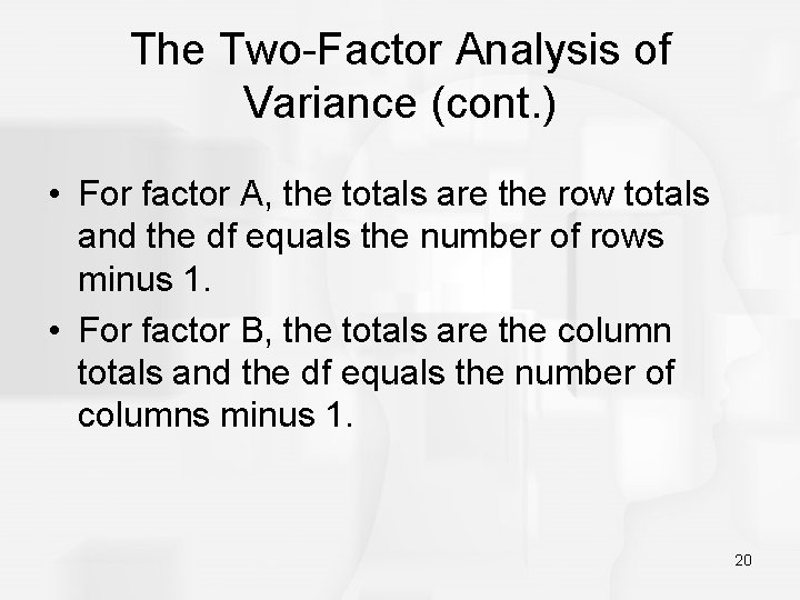
The Two-Factor Analysis of Variance (cont. ) • For factor A, the totals are the row totals and the df equals the number of rows minus 1. • For factor B, the totals are the column totals and the df equals the number of columns minus 1. 20

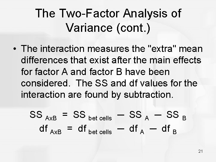
The Two-Factor Analysis of Variance (cont. ) • The interaction measures the "extra" mean differences that exist after the main effects for factor A and factor B have been considered. The SS and df values for the interaction are found by subtraction. SS Ax. B = SS bet cells ─ SS A ─ SS B df Ax. B = df bet cells ─ df A ─ df B 21