Chapter 15 Simulation Modeling To accompany Quantitative Analysis

Chapter 15 Simulation Modeling To accompany Quantitative Analysis for Management, Tenth Edition, by Render, Stair, and Hanna Power Point slides created by Jeff Heyl © 2008 Prentice-Hall, Inc. © 2009 Prentice-Hall, Inc.

Learning Objectives After completing this chapter, students will be able to: 1. Tackle a wide variety of problems by simulation 2. Understand the seven steps of conducting a simulation 3. Explain the advantages and disadvantages of simulation 4. Develop random number intervals and use them to generate outcomes 5. Understand alternative simulation packages available © 2009 Prentice-Hall, Inc. 15 – 2

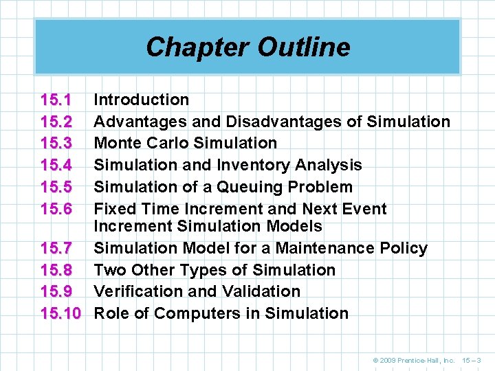
Chapter Outline 15. 1 15. 2 15. 3 15. 4 15. 5 15. 6 Introduction Advantages and Disadvantages of Simulation Monte Carlo Simulation and Inventory Analysis Simulation of a Queuing Problem Fixed Time Increment and Next Event Increment Simulation Models 15. 7 Simulation Model for a Maintenance Policy 15. 8 Two Other Types of Simulation 15. 9 Verification and Validation 15. 10 Role of Computers in Simulation © 2009 Prentice-Hall, Inc. 15 – 3

Introduction n Simulation is one of the most widely used n n quantitative analysis tools It is used by over half of the largest US corporations in corporate planning To simulate is to try to duplicate the features, appearance, and characteristics of a real system We will build a mathematical model that comes as close as possible to representing the reality of the system You can also build physical models to test systems © 2009 Prentice-Hall, Inc. 15 – 4

Introduction n The idea behind simulation is to imitate a real- world situation mathematically n Study its properties and operating characteristics n Draw conclusions and make action decisions © 2009 Prentice-Hall, Inc. 15 – 5

Introduction n Using simulation, a manager should 1. Define a problem 2. Introduce the variables associated with the problem 3. Construct a numerical model 4. Set up possible courses of action for testing 5. Run the experiment 6. Consider the results 7. Decide what courses of action to take © 2009 Prentice-Hall, Inc. 15 – 6

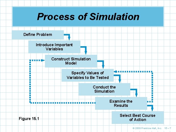
Process of Simulation Define Problem Introduce Important Variables Construct Simulation Model Specify Values of Variables to Be Tested Conduct the Simulation Examine the Results Figure 15. 1 Select Best Course of Action © 2009 Prentice-Hall, Inc. 15 – 7

Advantages and Disadvantages of Simulation n Simulation is useful because 1. It is relatively straightforward and flexible 2. Recent advances in computer software make simulation models very easy to develop 3. Can be used to analyze large and complex real-world situations 4. Allows “what-if? ” type questions 5. Does not interfere with the real-world system 6. Enables study of interactions between components 7. Enables time compression 8. Enables the inclusion of real-world © 2009 Prentice-Hall, Inc. complications 15 – 8

Advantages and Disadvantages of Simulation n The main disadvantages of simulation are 1. It is often expensive as it may require a long, complicated process to develop the model 2. Does not generate optimal solutions, it is a trial-and-error approach 3. Requires managers to generate all conditions and constraints of real-world problem 4. Each model is unique and the solutions and inferences are not usually transferable to other problems © 2009 Prentice-Hall, Inc. 15 – 9

Monte Carlo Simulation n When systems contain elements that exhibit chance in their behavior, the Monte Carlo method of simulation can be applied n Some examples are 1. Inventory demand 2. Lead time for inventory 3. Times between machine breakdowns 4. Times between arrivals 5. Service times 6. Times to complete project activities 7. Number of employees absent © 2009 Prentice-Hall, Inc. 15 – 10

Monte Carlo Simulation n The basis of the Monte Carlo simulation is experimentation on the probabilistic elements through random sampling n It is based on the following five steps 1. Setting up a probability distribution for important variables 2. Building a cumulative probability distribution for each variable 3. Establishing an interval of random numbers for each variable 4. Generating random numbers 5. Actually simulating a series of trials © 2009 Prentice-Hall, Inc. 15 – 11

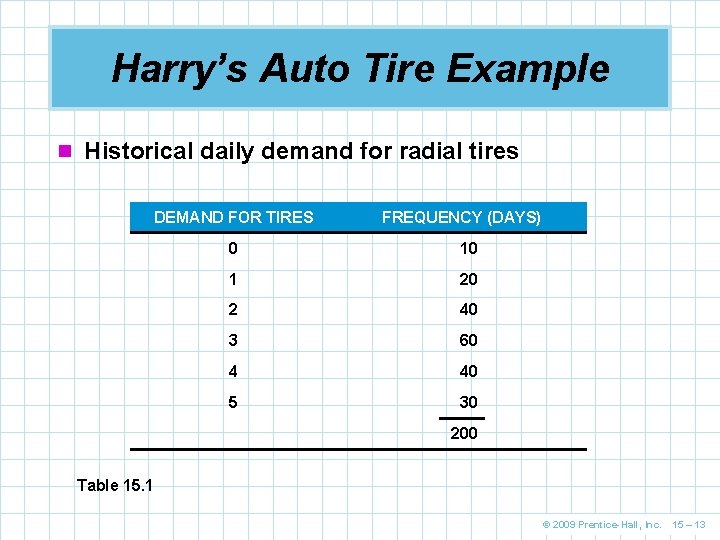
Harry’s Auto Tire Example n A popular radial tire accounts for a large portion of the sales at Harry’s Auto Tire n Harry wishes to determine a policy for managing this inventory n He wants to simulate the daily demand for a number of days Step 1: Establishing probability distributions n One way to establish a probability distribution for a given variable is to examine historical outcomes n Managerial estimates based on judgment and experience can also be used © 2009 Prentice-Hall, Inc. 15 – 12

Harry’s Auto Tire Example n Historical daily demand for radial tires DEMAND FOR TIRES FREQUENCY (DAYS) 0 10 1 20 2 40 3 60 4 40 5 30 200 Table 15. 1 © 2009 Prentice-Hall, Inc. 15 – 13

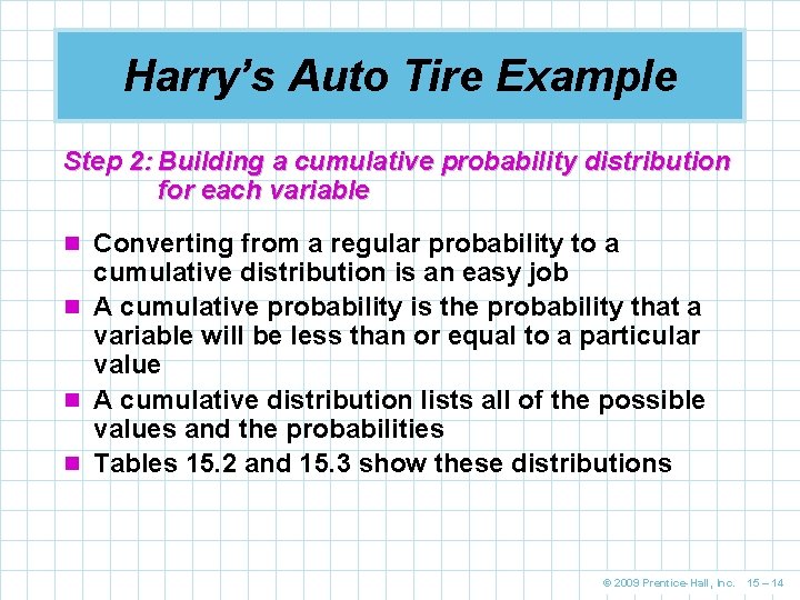
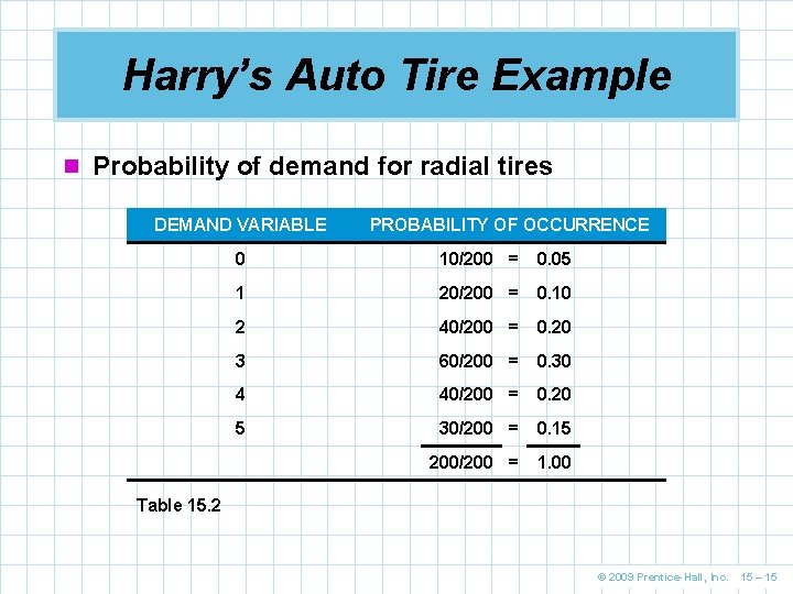
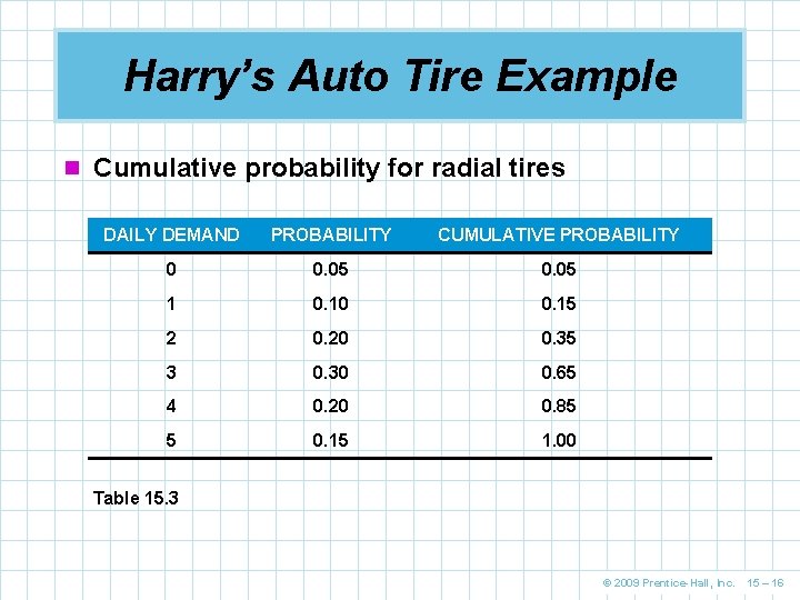
Harry’s Auto Tire Example Step 2: Building a cumulative probability distribution for each variable n Converting from a regular probability to a cumulative distribution is an easy job n A cumulative probability is the probability that a variable will be less than or equal to a particular value n A cumulative distribution lists all of the possible values and the probabilities n Tables 15. 2 and 15. 3 show these distributions © 2009 Prentice-Hall, Inc. 15 – 14

Harry’s Auto Tire Example n Probability of demand for radial tires DEMAND VARIABLE PROBABILITY OF OCCURRENCE 0 10/200 = 0. 05 1 20/200 = 0. 10 2 40/200 = 0. 20 3 60/200 = 0. 30 4 40/200 = 0. 20 5 30/200 = 0. 15 200/200 = 1. 00 Table 15. 2 © 2009 Prentice-Hall, Inc. 15 – 15

Harry’s Auto Tire Example n Cumulative probability for radial tires DAILY DEMAND PROBABILITY CUMULATIVE PROBABILITY 0 0. 05 1 0. 10 0. 15 2 0. 20 0. 35 3 0. 30 0. 65 4 0. 20 0. 85 5 0. 15 1. 00 Table 15. 3 © 2009 Prentice-Hall, Inc. 15 – 16

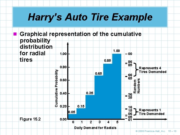
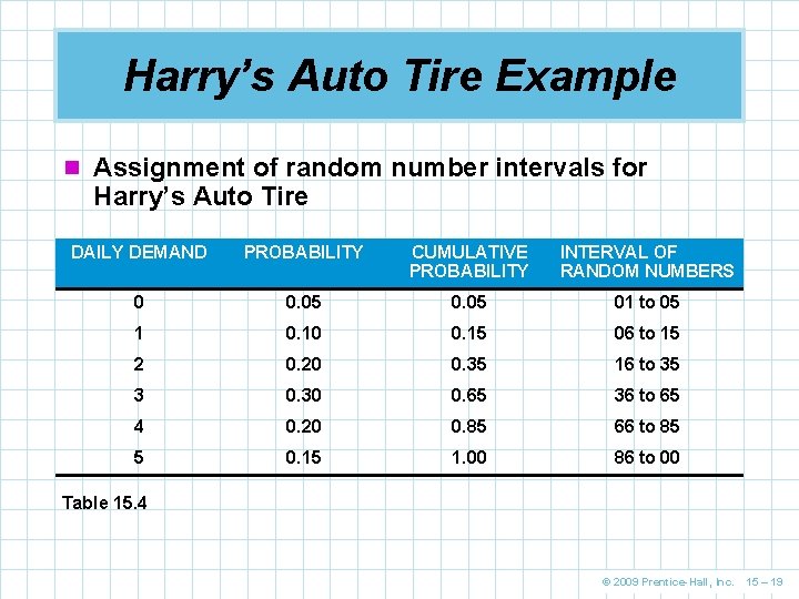
Harry’s Auto Tire Example Step 3: Setting random number intervals n We assign a set of numbers to represent each possible value or outcome n These are random number intervals n A random number is a series of digits that have been selected by a totally random process n The range of the random number intervals corresponds exactly to the probability of the outcomes as shown in Figure 15. 2 © 2009 Prentice-Hall, Inc. 15 – 17

Harry’s Auto Tire Example n Graphical representation of the cumulative 1. 00 – 0. 85 – 86 85 Cumulative Probability 0. 80 – 0. 65 – 66 65 0. 60 – 0. 35 0. 40 – – 36 35 0. 15 0. 20 – 0. 05 Figure 15. 2 0. 00 – 0 1 2 – 00 3 4 Daily Demand for Radials 5 – 16 15 06 – – 05 – 01 Represents 4 Tires Demanded Random Numbers probability distribution for radial tires Represents 1 Tire Demanded © 2009 Prentice-Hall, Inc. 15 – 18

Harry’s Auto Tire Example n Assignment of random number intervals for Harry’s Auto Tire DAILY DEMAND PROBABILITY CUMULATIVE PROBABILITY INTERVAL OF RANDOM NUMBERS 0 0. 05 01 to 05 1 0. 10 0. 15 06 to 15 2 0. 20 0. 35 16 to 35 3 0. 30 0. 65 36 to 65 4 0. 20 0. 85 66 to 85 5 0. 15 1. 00 86 to 00 Table 15. 4 © 2009 Prentice-Hall, Inc. 15 – 19

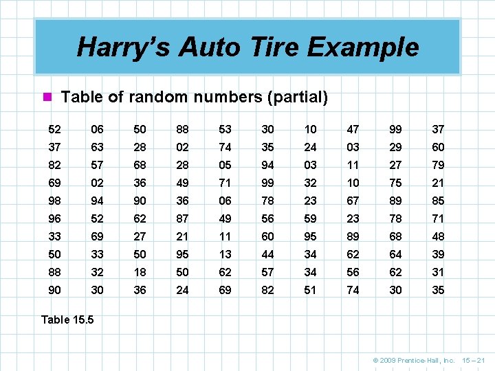
Harry’s Auto Tire Example Step 4: Generating random numbers n Random numbers can be generated in several ways n Large problems will use computer program to generate the needed random numbers n For small problems, random processes like roulette wheels or pulling chips from a hat may be used n The most common manual method is to use a random number table n Because everything is random in a random number table, we can select numbers from anywhere in the table to use in the simulation © 2009 Prentice-Hall, Inc. 15 – 20

Harry’s Auto Tire Example n Table of random numbers (partial) 52 06 50 88 53 30 10 47 99 37 37 63 28 02 74 35 24 03 29 60 82 57 68 28 05 94 03 11 27 79 69 02 36 49 71 99 32 10 75 21 98 94 90 36 06 78 23 67 89 85 96 52 62 87 49 56 59 23 78 71 33 69 27 21 11 60 95 89 68 48 50 33 50 95 13 44 34 62 64 39 88 32 18 50 62 57 34 56 62 31 90 30 36 24 69 82 51 74 30 35 Table 15. 5 © 2009 Prentice-Hall, Inc. 15 – 21

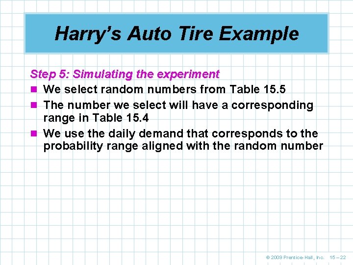
Harry’s Auto Tire Example Step 5: Simulating the experiment n We select random numbers from Table 15. 5 n The number we select will have a corresponding range in Table 15. 4 n We use the daily demand that corresponds to the probability range aligned with the random number © 2009 Prentice-Hall, Inc. 15 – 22

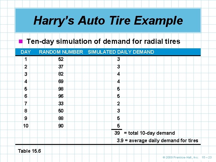
Harry’s Auto Tire Example n Ten-day simulation of demand for radial tires DAY RANDOM NUMBER SIMULATED DAILY DEMAND 1 52 3 2 37 3 3 82 4 4 69 4 5 98 5 6 96 5 7 33 2 8 50 3 9 88 5 10 90 5 39 = total 10 -day demand 3. 9 = average daily demand for tires Table 15. 6 © 2009 Prentice-Hall, Inc. 15 – 23

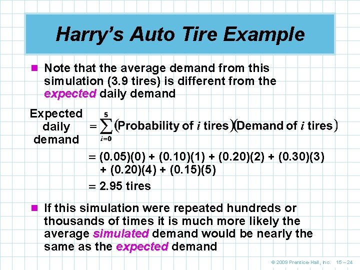
Harry’s Auto Tire Example n Note that the average demand from this simulation (3. 9 tires) is different from the expected daily demand Expected daily demand (0. 05)(0) + (0. 10)(1) + (0. 20)(2) + (0. 30)(3) + (0. 20)(4) + (0. 15)(5) 2. 95 tires n If this simulation were repeated hundreds or thousands of times it is much more likely the average simulated demand would be nearly the same as the expected demand © 2009 Prentice-Hall, Inc. 15 – 24

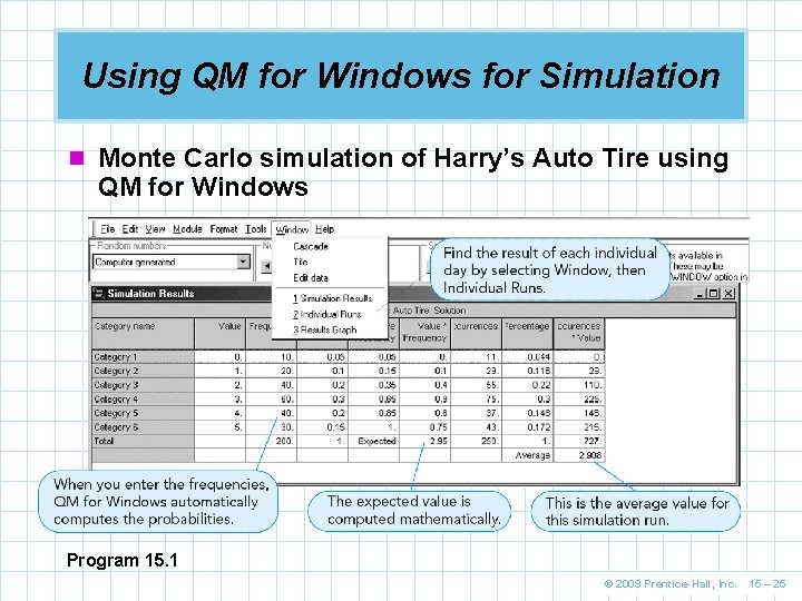
Using QM for Windows for Simulation n Monte Carlo simulation of Harry’s Auto Tire using QM for Windows Program 15. 1 © 2009 Prentice-Hall, Inc. 15 – 25

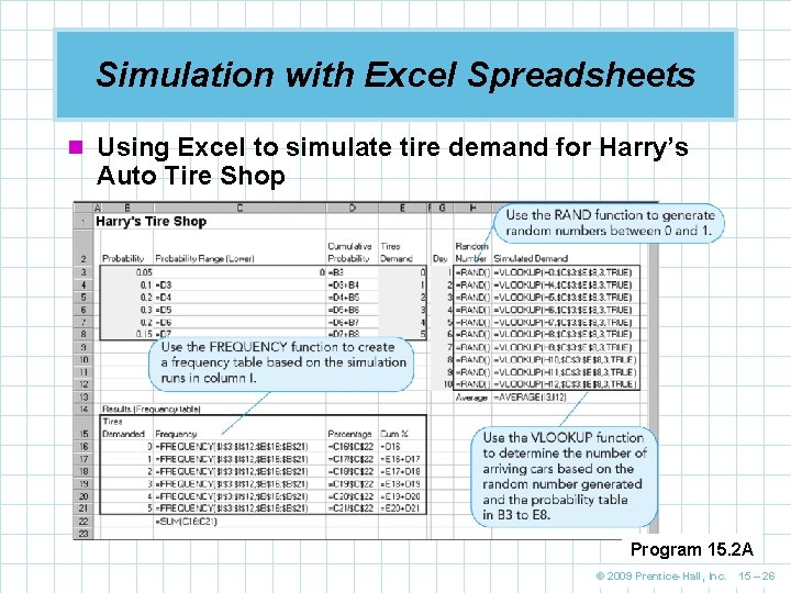
Simulation with Excel Spreadsheets n Using Excel to simulate tire demand for Harry’s Auto Tire Shop Program 15. 2 A © 2009 Prentice-Hall, Inc. 15 – 26

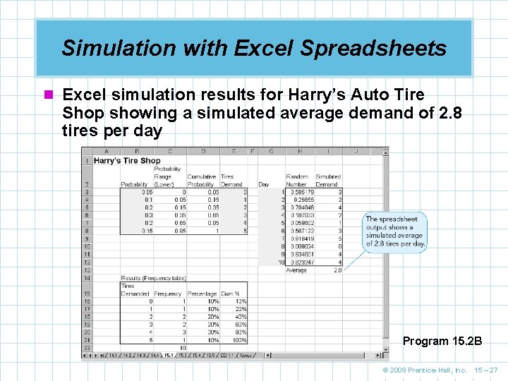
Simulation with Excel Spreadsheets n Excel simulation results for Harry’s Auto Tire Shop showing a simulated average demand of 2. 8 tires per day Program 15. 2 B © 2009 Prentice-Hall, Inc. 15 – 27

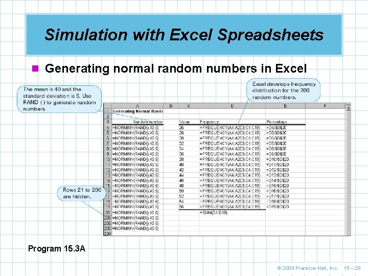
Simulation with Excel Spreadsheets n Generating normal random numbers in Excel Program 15. 3 A © 2009 Prentice-Hall, Inc. 15 – 28

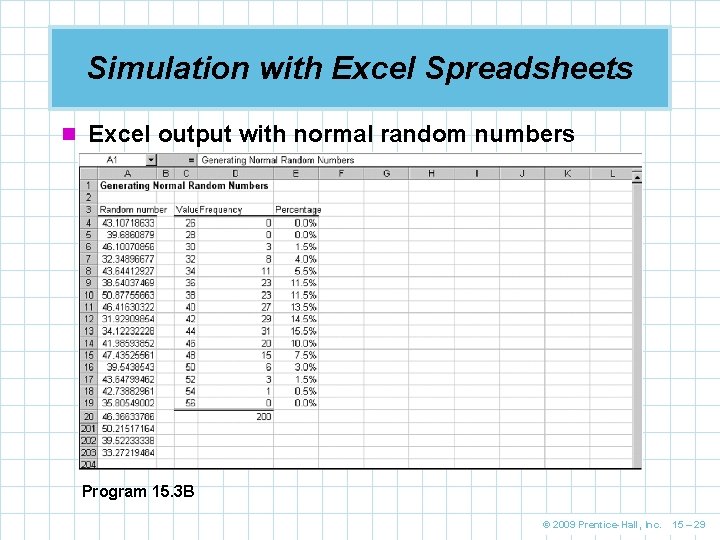
Simulation with Excel Spreadsheets n Excel output with normal random numbers Program 15. 3 B © 2009 Prentice-Hall, Inc. 15 – 29

Simulation and Inventory Analysis n We have seen deterministic inventory models n In many real-world inventory situations, demand lead time are variables n Accurate analysis is difficult without simulation n We will look at an inventory problem with two decision variables and two probabilistic components n The owner of a hardware store wants to establish order quantity and reorder point decisions for a product that has probabilistic daily demand reorder lead time © 2009 Prentice-Hall, Inc. 15 – 30

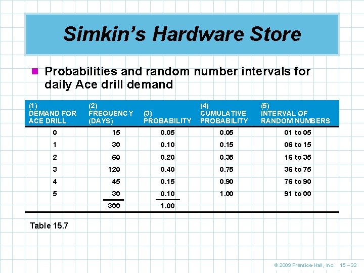
Simkin’s Hardware Store n The owner of a hardware store wants to find a n n good, low cost inventory policy for an electric drill Simkin identifies two types of variables, controllable and uncontrollable inputs The controllable inputs are the order quantity and reorder points The uncontrollable inputs are daily demand variable lead time The demand data for the drill is shown in Table 15. 7 © 2009 Prentice-Hall, Inc. 15 – 31

Simkin’s Hardware Store n Probabilities and random number intervals for daily Ace drill demand (1) DEMAND FOR ACE DRILL (2) FREQUENCY (DAYS) (3) PROBABILITY (4) CUMULATIVE PROBABILITY (5) INTERVAL OF RANDOM NUMBERS 0 15 0. 05 01 to 05 1 30 0. 15 06 to 15 2 60 0. 20 0. 35 16 to 35 3 120 0. 40 0. 75 36 to 75 4 45 0. 15 0. 90 76 to 90 5 30 0. 10 1. 00 91 to 00 300 1. 00 Table 15. 7 © 2009 Prentice-Hall, Inc. 15 – 32

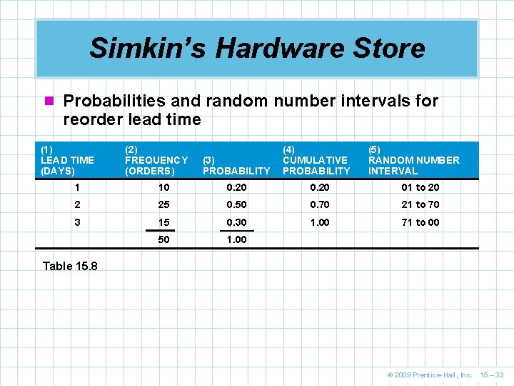
Simkin’s Hardware Store n Probabilities and random number intervals for reorder lead time (1) LEAD TIME (DAYS) (2) FREQUENCY (ORDERS) (3) PROBABILITY (4) CUMULATIVE PROBABILITY (5) RANDOM NUMBER INTERVAL 1 10 0. 20 01 to 20 2 25 0. 50 0. 70 21 to 70 3 15 0. 30 1. 00 71 to 00 50 1. 00 Table 15. 8 © 2009 Prentice-Hall, Inc. 15 – 33

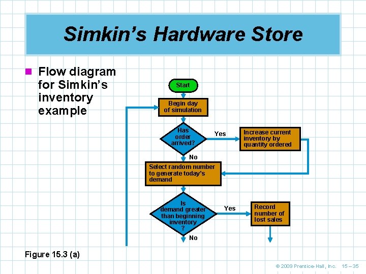
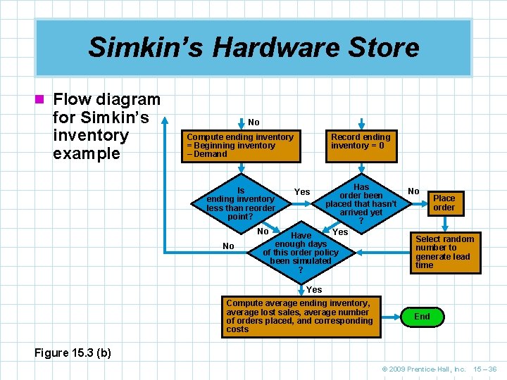
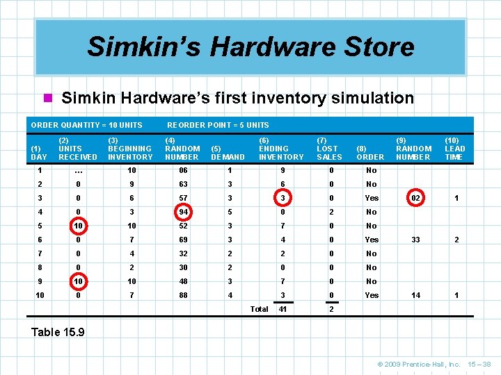
Simkin’s Hardware Store n The third step is to develop a simulation model n A flow diagram, or flowchart, is helpful in this n n process The fourth step in the process is to specify the values of the variables that we wish to test The first policy Simkin wants to test is an order quantity of 10 with a reorder point of 5 The fifth step is to actually conduct the simulation The process is simulated for a 10 day period © 2009 Prentice-Hall, Inc. 15 – 34

Simkin’s Hardware Store n Flow diagram for Simkin’s inventory example Start Begin day of simulation Has order arrived? Yes Increase current inventory by quantity ordered No Select random number to generate today’s demand Is demand greater than beginning inventory ? Yes Record number of lost sales No Figure 15. 3 (a) © 2009 Prentice-Hall, Inc. 15 – 35

Simkin’s Hardware Store n Flow diagram for Simkin’s inventory example No Compute ending inventory = Beginning inventory – Demand Has order been placed that hasn’t arrived yet ? No Yes Have enough days of this order policy been simulated ? Is ending inventory less than reorder point? No Record ending inventory = 0 Yes No Place order Select random number to generate lead time Yes Compute average ending inventory, average lost sales, average number of orders placed, and corresponding costs End Figure 15. 3 (b) © 2009 Prentice-Hall, Inc. 15 – 36

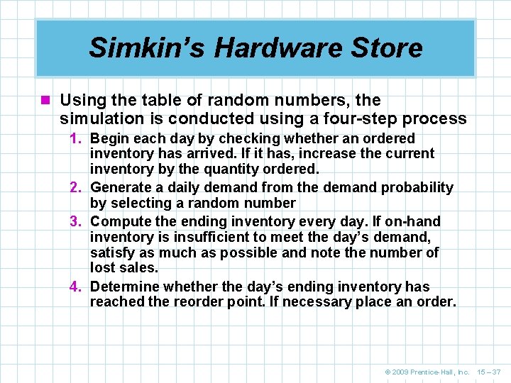
Simkin’s Hardware Store n Using the table of random numbers, the simulation is conducted using a four-step process 1. Begin each day by checking whether an ordered inventory has arrived. If it has, increase the current inventory by the quantity ordered. 2. Generate a daily demand from the demand probability by selecting a random number 3. Compute the ending inventory every day. If on-hand inventory is insufficient to meet the day’s demand, satisfy as much as possible and note the number of lost sales. 4. Determine whether the day’s ending inventory has reached the reorder point. If necessary place an order. © 2009 Prentice-Hall, Inc. 15 – 37

Simkin’s Hardware Store n Simkin Hardware’s first inventory simulation ORDER QUANTITY = 10 UNITS REORDER POINT = 5 UNITS (1) DAY (2) UNITS RECEIVED (3) BEGINNING INVENTORY (4) RANDOM NUMBER (5) DEMAND (6) ENDING INVENTORY (7) LOST SALES (8) ORDER 1 … 10 06 1 9 0 No 2 0 9 63 3 6 0 No 3 0 6 57 3 3 0 Yes 4 0 3 94 5 0 2 No 5 10 10 52 3 7 0 No 6 0 7 69 3 4 0 Yes 7 0 4 32 2 2 0 No 8 0 2 30 2 0 0 No 9 10 10 48 3 7 0 No 10 0 7 88 4 3 0 Yes 41 2 Total (9) RANDOM NUMBER (10) LEAD TIME 02 1 33 2 14 1 Table 15. 9 © 2009 Prentice-Hall, Inc. 15 – 38

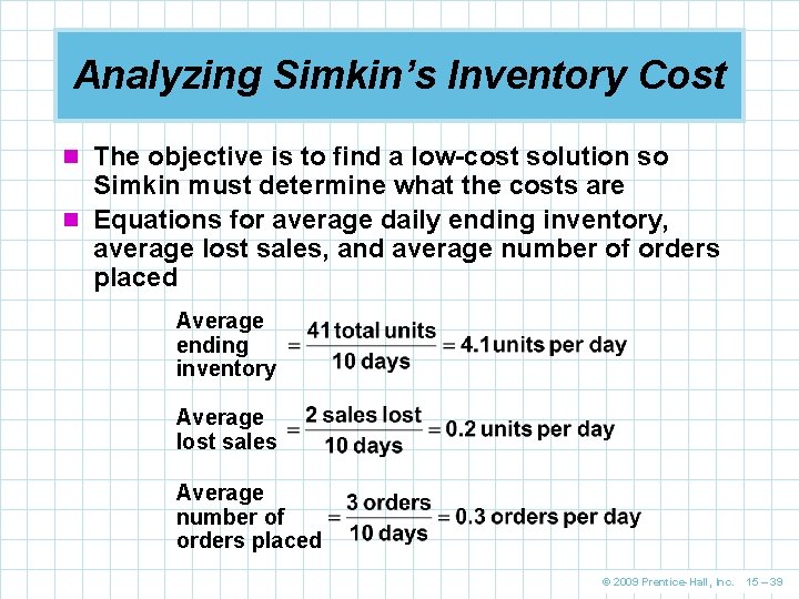
Analyzing Simkin’s Inventory Cost n The objective is to find a low-cost solution so Simkin must determine what the costs are n Equations for average daily ending inventory, average lost sales, and average number of orders placed Average ending inventory Average lost sales Average number of orders placed © 2009 Prentice-Hall, Inc. 15 – 39

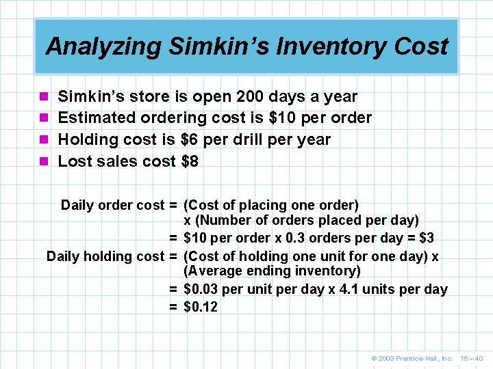
Analyzing Simkin’s Inventory Cost n Simkin’s store is open 200 days a year n Estimated ordering cost is $10 per order n Holding cost is $6 per drill per year n Lost sales cost $8 Daily order cost = (Cost of placing one order) x (Number of orders placed per day) = $10 per order x 0. 3 orders per day = $3 Daily holding cost = (Cost of holding one unit for one day) x (Average ending inventory) = $0. 03 per unit per day x 4. 1 units per day = $0. 12 © 2009 Prentice-Hall, Inc. 15 – 40

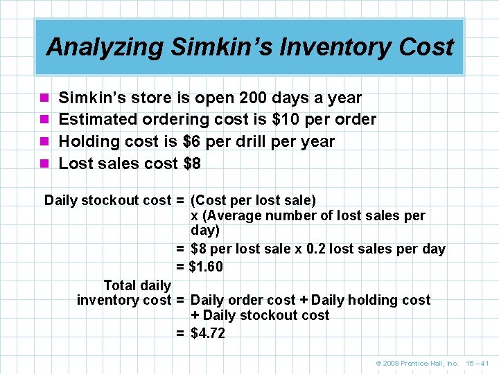
Analyzing Simkin’s Inventory Cost n Simkin’s store is open 200 days a year n Estimated ordering cost is $10 per order n Holding cost is $6 per drill per year n Lost sales cost $8 Daily stockout cost = (Cost per lost sale) x (Average number of lost sales per day) = $8 per lost sale x 0. 2 lost sales per day = $1. 60 Total daily inventory cost = Daily order cost + Daily holding cost + Daily stockout cost = $4. 72 © 2009 Prentice-Hall, Inc. 15 – 41

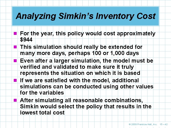
Analyzing Simkin’s Inventory Cost n For the year, this policy would cost approximately n n $944 This simulation should really be extended for many more days, perhaps 100 or 1, 000 days Even after a larger simulation, the model must be verified and validated to make sure it truly represents the situation on which it is based If we are satisfied with the model, additional simulations can be conducted using other values for the variables After simulating all reasonable combinations, Simkin would select the policy that results in the lowest total cost © 2009 Prentice-Hall, Inc. 15 – 42

Simulation of a Queuing Problem n Modeling waiting lines is an important application of simulation n The assumptions of queuing models are quite restrictive n Sometimes simulation is the only approach that fits n In this example, arrivals do not follow a Poisson distribution and unloading rates are not exponential or constant © 2009 Prentice-Hall, Inc. 15 – 43

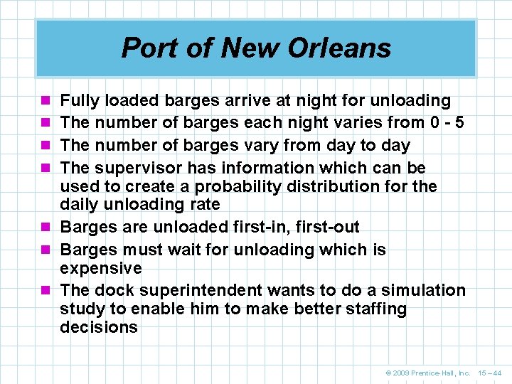
Port of New Orleans n Fully loaded barges arrive at night for unloading n The number of barges each night varies from 0 - 5 n The number of barges vary from day to day n The supervisor has information which can be used to create a probability distribution for the daily unloading rate n Barges are unloaded first-in, first-out n Barges must wait for unloading which is expensive n The dock superintendent wants to do a simulation study to enable him to make better staffing decisions © 2009 Prentice-Hall, Inc. 15 – 44

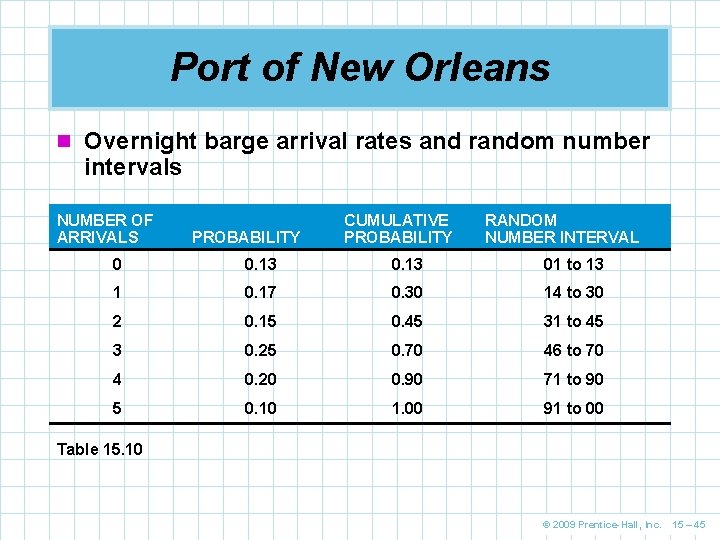
Port of New Orleans n Overnight barge arrival rates and random number intervals NUMBER OF ARRIVALS PROBABILITY CUMULATIVE PROBABILITY RANDOM NUMBER INTERVAL 0 0. 13 01 to 13 1 0. 17 0. 30 14 to 30 2 0. 15 0. 45 31 to 45 3 0. 25 0. 70 46 to 70 4 0. 20 0. 90 71 to 90 5 0. 10 1. 00 91 to 00 Table 15. 10 © 2009 Prentice-Hall, Inc. 15 – 45

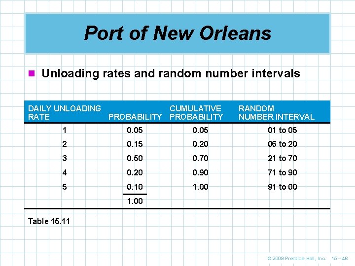
Port of New Orleans n Unloading rates and random number intervals DAILY UNLOADING CUMULATIVE RATE PROBABILITY RANDOM NUMBER INTERVAL 1 0. 05 01 to 05 2 0. 15 0. 20 06 to 20 3 0. 50 0. 70 21 to 70 4 0. 20 0. 90 71 to 90 5 0. 10 1. 00 91 to 00 1. 00 Table 15. 11 © 2009 Prentice-Hall, Inc. 15 – 46

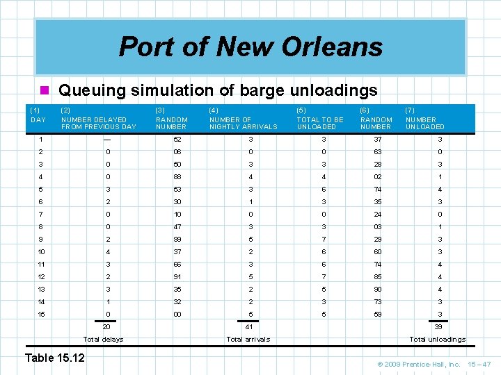
Port of New Orleans n Queuing simulation of barge unloadings (1) DAY (2) NUMBER DELAYED FROM PREVIOUS DAY (3) RANDOM NUMBER (4) NUMBER OF NIGHTLY ARRIVALS (5) TOTAL TO BE UNLOADED (6) RANDOM NUMBER (7) NUMBER UNLOADED 1 — 52 3 3 37 3 2 0 06 0 0 63 0 50 3 3 28 3 4 0 88 4 4 02 1 5 3 53 3 6 74 4 6 2 30 1 3 35 3 7 0 10 0 0 24 0 8 0 47 3 3 03 1 9 2 99 5 7 29 3 10 4 37 2 6 60 3 11 3 66 3 6 74 4 12 2 91 5 7 85 4 13 3 35 2 5 90 4 14 1 32 2 3 73 3 15 0 00 5 5 59 3 20 Total delays Table 15. 12 41 39 Total arrivals Total unloadings © 2009 Prentice-Hall, Inc. 15 – 47

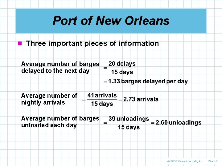
Port of New Orleans n Three important pieces of information Average number of barges delayed to the next day Average number of nightly arrivals Average number of barges unloaded each day © 2009 Prentice-Hall, Inc. 15 – 48

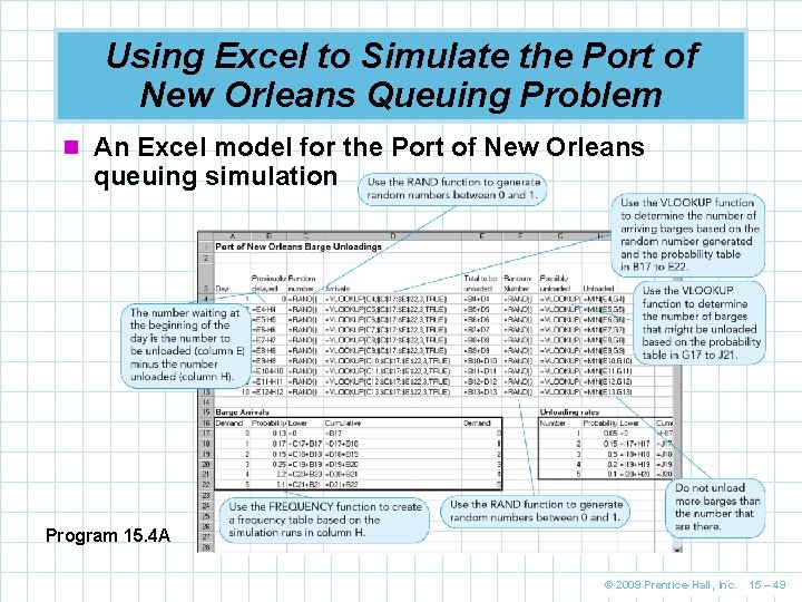
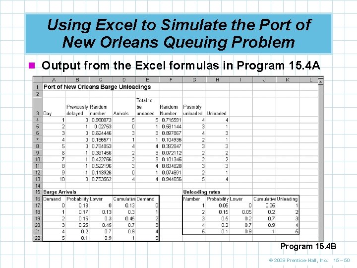
Using Excel to Simulate the Port of New Orleans Queuing Problem n An Excel model for the Port of New Orleans queuing simulation Program 15. 4 A © 2009 Prentice-Hall, Inc. 15 – 49

Using Excel to Simulate the Port of New Orleans Queuing Problem n Output from the Excel formulas in Program 15. 4 A Program 15. 4 B © 2009 Prentice-Hall, Inc. 15 – 50

Fixed Time Increment and Next Event Increment Simulation Models n Simulation models are often classified into fixed n n n time increment models and next event increment models The terms refer to the frequency in which the system status is updated Fixed time increments update the status of the system at fixed time intervals Next event increment models update only when the system status changes Fixed event models randomly generate the number of events that occur during a time period Next event models randomly generate the time that elapses until the next event occurs © 2009 Prentice-Hall, Inc. 15 – 51

Simulation Model for a Maintenance Policy n Simulation can be used to analyze different maintenance policies before actually implementing them n Many options regarding staffing levels, parts replacement schedules, downtime, and labor costs can be compared n This can including completely shutting down factories for maintenance © 2009 Prentice-Hall, Inc. 15 – 52

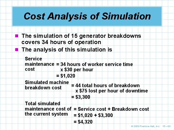
Three Hills Power Company n Three Hills provides power to a large city through a series of almost 200 electric generators n The company is concerned about generator failures because a breakdown costs about $75 per generator per hour n Their four repair people earn $30 per hour and work rotating 8 hour shifts n Management wants to evaluate the 1. Service maintenance cost 2. Simulated machine breakdown cost 3. Total cost © 2009 Prentice-Hall, Inc. 15 – 53

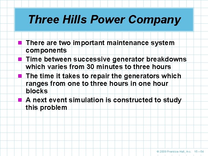
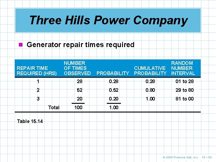
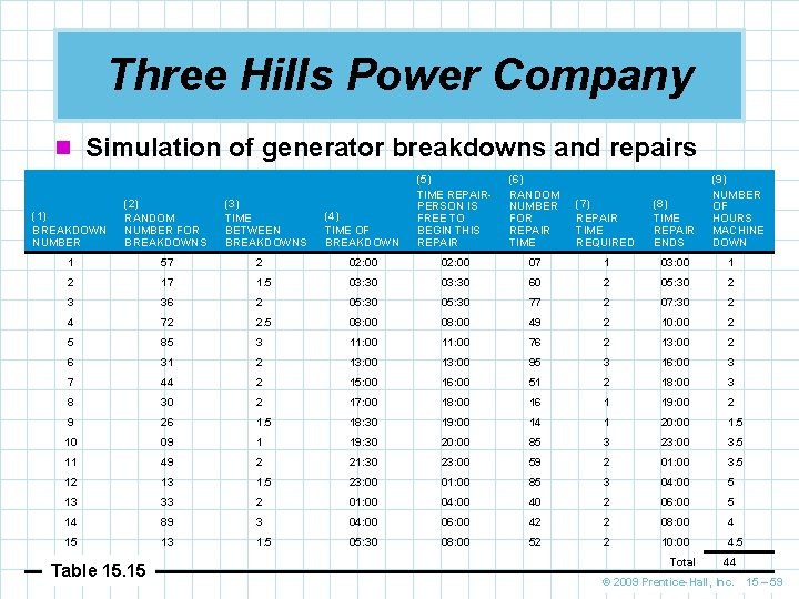
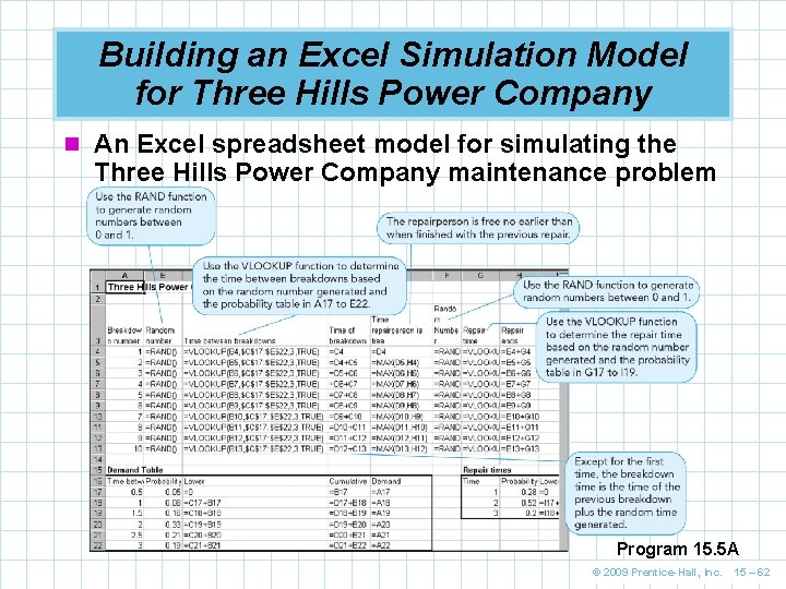
Three Hills Power Company n There are two important maintenance system components n Time between successive generator breakdowns which varies from 30 minutes to three hours n The time it takes to repair the generators which ranges from one to three hours in one hour blocks n A next event simulation is constructed to study this problem © 2009 Prentice-Hall, Inc. 15 – 54

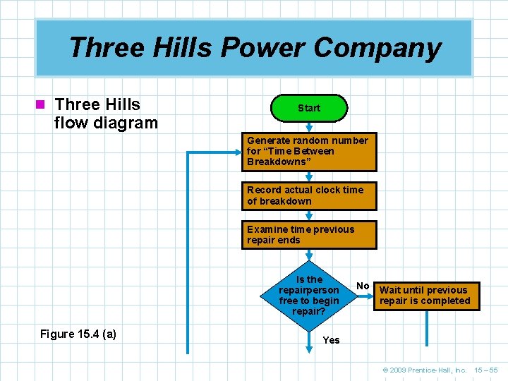
Three Hills Power Company n Three Hills flow diagram Start Generate random number for “Time Between Breakdowns” Record actual clock time of breakdown Examine time previous repair ends Is the repairperson free to begin repair? Figure 15. 4 (a) No Wait until previous repair is completed Yes © 2009 Prentice-Hall, Inc. 15 – 55

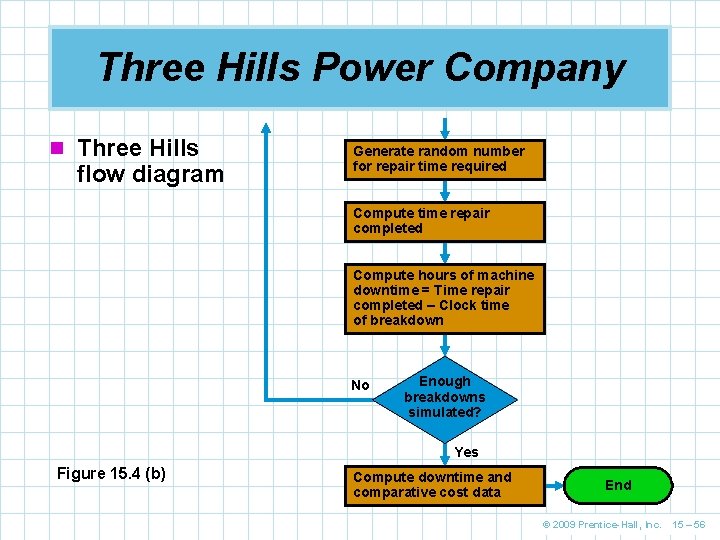
Three Hills Power Company n Three Hills flow diagram Generate random number for repair time required Compute time repair completed Compute hours of machine downtime = Time repair completed – Clock time of breakdown No Enough breakdowns simulated? Yes Figure 15. 4 (b) Compute downtime and comparative cost data End © 2009 Prentice-Hall, Inc. 15 – 56

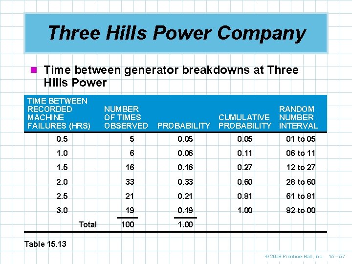
Three Hills Power Company n Time between generator breakdowns at Three Hills Power TIME BETWEEN RECORDED MACHINE FAILURES (HRS) NUMBER OF TIMES OBSERVED PROBABILITY RANDOM CUMULATIVE NUMBER PROBABILITY INTERVAL 0. 5 5 0. 05 01 to 05 1. 0 6 0. 06 0. 11 06 to 11 1. 5 16 0. 27 12 to 27 2. 0 33 0. 60 28 to 60 2. 5 21 0. 81 61 to 81 3. 0 19 0. 19 1. 00 82 to 00 1. 00 Total Table 15. 13 © 2009 Prentice-Hall, Inc. 15 – 57

Three Hills Power Company n Generator repair times required REPAIR TIME REQUIRED (HRS) NUMBER OF TIMES OBSERVED PROBABILITY RANDOM CUMULATIVE NUMBER PROBABILITY INTERVAL 1 28 01 to 28 2 52 0. 80 29 to 80 3 20 0. 20 1. 00 81 to 00 1. 00 Total Table 15. 14 © 2009 Prentice-Hall, Inc. 15 – 58

Three Hills Power Company n Simulation of generator breakdowns and repairs (4) TIME OF BREAKDOWN (6) RANDOM NUMBER FOR REPAIR TIME (7) REPAIR TIME REQUIRED (8) TIME REPAIR ENDS (9) NUMBER OF HOURS MACHINE DOWN (1) BREAKDOWN NUMBER (2) RANDOM NUMBER FOR BREAKDOWNS 1 57 2 02: 00 07 1 03: 00 1 2 17 1. 5 03: 30 60 2 05: 30 2 3 36 2 05: 30 77 2 07: 30 2 4 72 2. 5 08: 00 49 2 10: 00 2 5 85 3 11: 00 76 2 13: 00 2 6 31 2 13: 00 95 3 16: 00 3 7 44 2 15: 00 16: 00 51 2 18: 00 3 8 30 2 17: 00 18: 00 16 1 19: 00 2 9 26 1. 5 18: 30 19: 00 14 1 20: 00 1. 5 10 09 1 19: 30 20: 00 85 3 23: 00 3. 5 11 49 2 21: 30 23: 00 59 2 01: 00 3. 5 12 13 1. 5 23: 00 01: 00 85 3 04: 00 5 13 33 2 01: 00 04: 00 40 2 06: 00 5 14 89 3 04: 00 06: 00 42 2 08: 00 4 15 13 1. 5 05: 30 08: 00 52 2 10: 00 4. 5 Table 15. 15 (3) TIME BETWEEN BREAKDOWNS (5) TIME REPAIRPERSON IS FREE TO BEGIN THIS REPAIR Total 44 © 2009 Prentice-Hall, Inc. 15 – 59

Cost Analysis of Simulation n The simulation of 15 generator breakdowns covers 34 hours of operation n The analysis of this simulation is Service maintenance = 34 hours of worker service time cost x $30 per hour = $1, 020 Simulated machine = 44 total hours of breakdown cost x $75 lost per hour of downtime = $3, 300 Total simulated maintenance cost of = Service cost + Breakdown cost the current system = $1, 020 + $3, 300 = $4, 320 © 2009 Prentice-Hall, Inc. 15 – 60

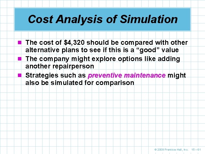
Cost Analysis of Simulation n The cost of $4, 320 should be compared with other alternative plans to see if this is a “good” value n The company might explore options like adding another repairperson n Strategies such as preventive maintenance might also be simulated for comparison © 2009 Prentice-Hall, Inc. 15 – 61

Building an Excel Simulation Model for Three Hills Power Company n An Excel spreadsheet model for simulating the Three Hills Power Company maintenance problem Program 15. 5 A © 2009 Prentice-Hall, Inc. 15 – 62

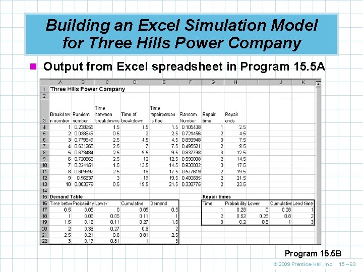
Building an Excel Simulation Model for Three Hills Power Company n Output from Excel spreadsheet in Program 15. 5 A Program 15. 5 B © 2009 Prentice-Hall, Inc. 15 – 63

Two Other Types of Simulation Models n Simulation models are often broken into three categories n The Monte Carlo method n Operational gaming n Systems simulation n Though theoretically different, computerized simulation has tended to blur the differences © 2009 Prentice-Hall, Inc. 15 – 64

Operational Gaming n Operational gaming refers to simulation involving two or more competing players n The best examples of this are military games and business games n These types of simulation allow the testing of skills and decision-making in a competitive environment © 2009 Prentice-Hall, Inc. 15 – 65

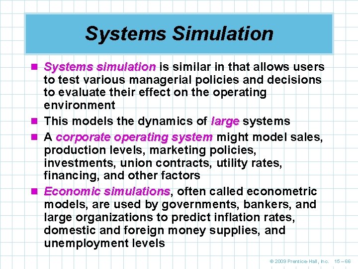
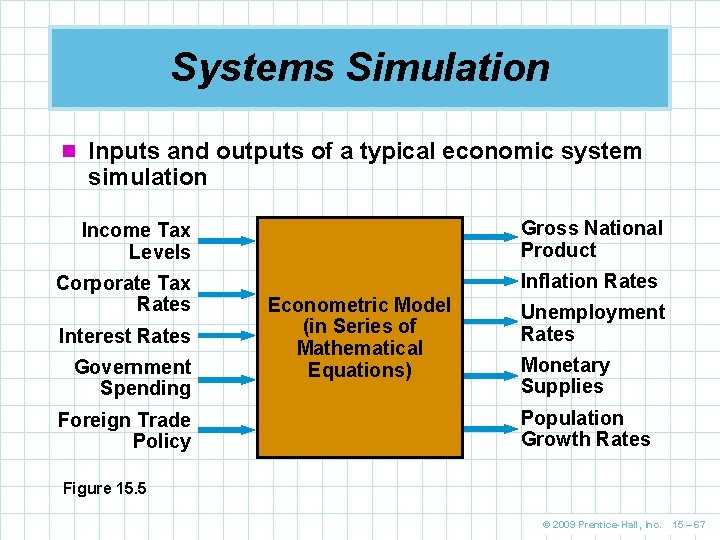
Systems Simulation n Systems simulation is similar in that allows users to test various managerial policies and decisions to evaluate their effect on the operating environment n This models the dynamics of large systems n A corporate operating system might model sales, production levels, marketing policies, investments, union contracts, utility rates, financing, and other factors n Economic simulations, simulations often called econometric models, are used by governments, bankers, and large organizations to predict inflation rates, domestic and foreign money supplies, and unemployment levels © 2009 Prentice-Hall, Inc. 15 – 66

Systems Simulation n Inputs and outputs of a typical economic system simulation Income Tax Levels Gross National Product Corporate Tax Rates Inflation Rates Interest Rates Government Spending Foreign Trade Policy Econometric Model (in Series of Mathematical Equations) Unemployment Rates Monetary Supplies Population Growth Rates Figure 15. 5 © 2009 Prentice-Hall, Inc. 15 – 67

Verification and Validation n It is important that a simulation model be checked n n to see that it is working properly and providing good representation of the real world situation The verification process involves determining that the computer model is internally consistent and following the logic of the conceptual model Verification answers the question “Did we build the model right? ” Validation is the process of comparing a simulation model to the real system it represents to make sure it is accurate Validation answers the question “Did we build the right model? ” © 2009 Prentice-Hall, Inc. 15 – 68

Role of Computers in Simulation n Computers are critical in simulating complex tasks n Three types of computer programming languages are available to help the simulation process n General-purpose languages n Special-purpose simulation languages 1. These require less programming 2. Are more efficient and easier to check for errors 3. Have random number generators built in n Pre-written simulation programs built to handle a wide range of common problems n Excel and add-ins can also be used for simulation problems © 2009 Prentice-Hall, Inc. 15 – 69