CHAPTER 15 Sampling Distributions Basic Practice of Statistics

CHAPTER 15: Sampling Distributions Basic Practice of Statistics 7 th Edition Lecture Power. Point Slides

In Chapter 15, we cover … �
 �")
Sampling Terminology (Parameters and statistics) �

Parameter vs Statistic A properly chosen sample of 1600 people across the United States was asked if they regularly watch a certain television program, and 24% said yes. The parameter of interest here is the true proportion of all people in the U. S. who watch the program, while the statistic is the value 24% obtained from the sample of 1600 people.

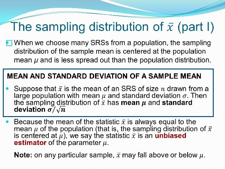
Parameter vs. Statistic u. The mean of a population is denoted by µ – this is a parameter. u. The mean of a sample is denoted by – this is a statistic. is used to estimate µ. u. The true proportion of a population with a certain trait is denoted by p – this is a parameter. u. The proportion of a sample with a certain trait is denoted by (“p-hat”) – this is a statistic. is used to estimate p.
 A parameter is a number that describes the")
Parameters and Statistics (1 of 2) A parameter is a number that describes the _____. a) population b) sample c) statistic d) None of the answer options is correct.
 A ______ is a number that can be")
Parameters and Statistics (2 of 2) A ______ is a number that can be computed from the sample data to estimate an unknown population parameter. a) population b) parameter c) statistic d) None of the answer options is correct.

Statistical estimation � The process of statistical inference involves using information from a sample to draw conclusions about a wider population. � Different random samples yield different statistics. We need to be able to describe the sampling distribution of possible statistic values in order to perform statistical inference. � We can think of a statistic as a random variable because it takes numerical values that describe the outcomes of the random sampling process. Therefore, we can examine its probability distribution using concepts we learned in earlier chapters. Population Sample Collect data from a representative sample Make an inference about the population

The law of large numbers �
 �The “house” in a gambling operation is not")
The Law of Large Numbers (Gambling) �The “house” in a gambling operation is not gambling at all �the games are defined so that the gambler has a negative expected gain per play (the true mean gain is negative) �each play is independent of previous plays, so the law of large numbers guarantees that the average winnings of a large number of customers will be close the (negative) true average
 As the sample size gets larger, the")
Law of Large Numbers (1 of 2) As the sample size gets larger, the sample mean gets closer to the ____. a) population mean b) population variance c) population standard deviation d) population median
 �")
Law of Large Numbers (2 of 2) �

Sampling distributions �

Population distributions vs. sampling distributions
 is sometimes present in")
Case Study Does This Wine Smell Bad? Dimethyl sulfide (DMS) is sometimes present in wine, causing “off-odors”. Winemakers want to know the odor threshold – the lowest concentration of DMS that the human nose can detect. Different people have different thresholds, and of interest is the mean threshold in the population of all adults.

Case Study Does This Wine Smell Bad? Suppose the mean threshold of all adults is =25 micrograms of DMS per liter of wine, with a standard deviation of =7 micrograms per liter and the threshold values follow a bell-shaped (normal) curve.

Where should 95% of all individual threshold values fall? �mean plus or minus two standard deviations 25 2(7) = 11 25 + 2(7) = 39 � 95% should fall between 11 & 39 �What about the mean (average) of a sample of 10 adults? What values would be expected?
 of a sample of 10 adults? What")
Sampling Distribution �What about the mean (average) of a sample of 10 adults? What values would be expected? u Answer this by thinking: “What would happen if we took many samples of 10 subjects from this population? ” – take a large number of samples of 10 subjects from the population – calculate the sample mean (x-bar) for each sample – make a histogram of the values of x-bar – examine the graphical display for shape, center, spread

Case Study Does This Wine Smell Bad? Mean threshold of all adults is =25 micrograms per liter, with a standard deviation of =7 micrograms per liter and the threshold values follow a bell-shaped (normal) curve. Many (1000) samples of n=10 adults from the population were taken and the resulting histogram of the 1000 x-bar values is on the next slide.

Does This Wine Smell Bad?
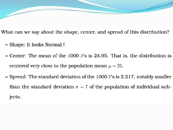

Case Study Does This Wine Smell Bad? Mean threshold of all adults is =25 with a standard deviation of =7, and the threshold values follow a bell-shaped (normal) curve. (Population distribution)
 The sampling distribution of a statistic is the distribution")
Sampling Distribution (1 of 3) The sampling distribution of a statistic is the distribution of values taken by the statistic in all possible samples of the same size from different populations. a) true b) false
 ______ is “correct on the average” in many samples.")
Sampling Distributions (2 of 3) ______ is “correct on the average” in many samples. How close the estimator falls to the parameter in most samples is determined by the _____ of the sampling distribution. a) An unbiased estimator; spread/variability b) The law of large numbers; mean c) An unbiased estimator; mean d) The law of large numbers; median
 �")
Sampling Distributions (3 of 3) �

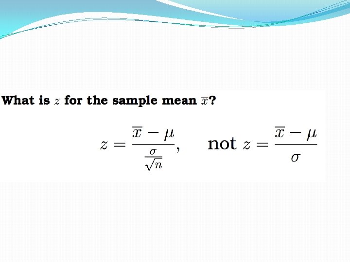
Standard Deviation of Sample Mean �

The central limit theorem �
")
Central limit theorem: example (part I)
 Normal curve from the central limit theorem")
Central limit theorem: example (part II) Normal curve from the central limit theorem

Central Limit Theorem: Sample Size u How large must n be for the CLT to hold? – depends on how far the population distribution is from Normal v the further from Normal, the larger the sample size needed v a sample size of 25 or 30 is typically large enough for any population distribution encountered in practice v recall: if the population is Normal, any sample size will work (n≥ 1)

n=1 n=2 n=10 n=25
 �")
Central Limit Theorem (1 of 2) �
 A sample of size 64 is taken from")
Central Limit Theorem (2 of 2) A sample of size 64 is taken from a distribution with mean 100 and standard deviation 24. The sample mean will have a distribution that is approximately _______ with standard deviation ______. a) Normal; 24/64 b) binomial; 24/64 c) Normal; 24/8 d) binomial; 24/8
- Slides: 40