CHAPTER 15 NONPARAMETRIC STATISTICS Learning Objectives Determine situations

CHAPTER 15 NONPARAMETRIC STATISTICS

Learning Objectives • Determine situations where nonparametric procedures are better alternatives to the parametric tests • Understand the assumptions of nonparametric tests • Use one- and two-sample nonparametric tests • Use nonparametric alternatives to the single-factor ANOVA

Nonparametric vs. Parametric • Used an assumption that we are working with random samples from normal populations • Called parametric methods • Based on a particular parametric family of distributions • Describe procedures called nonparametric methods • Make no assumptions about the population distribution other than that it is continuous

Why Nonparametric Procedures • Distributions are not close to normal • Data need not be quantitative but can be categorical (such as yes or no, defective or non defective) or rank data • Are usually very quick and easy to perform • Provides considerable improvement over the normal-theory parametric methods • Not utilize all the information provided by the sample • Requirement of a larger sample size

Which One? • Which one to choose? • If both methods are applicable to a particular problem • Use the more efficient parametric procedure • Otherwise, use the non parametric procedure

SIGN TEST • Used to test hypotheses about the median of a continuous distribution • Mean of a normal distribution equals the median • Sign test can be used to test hypotheses about the mean of a normal distribution • Used the t-test in Chapter 9 • Sign test is appropriate for samples from any continuous distribution • Counterpart of the t-test

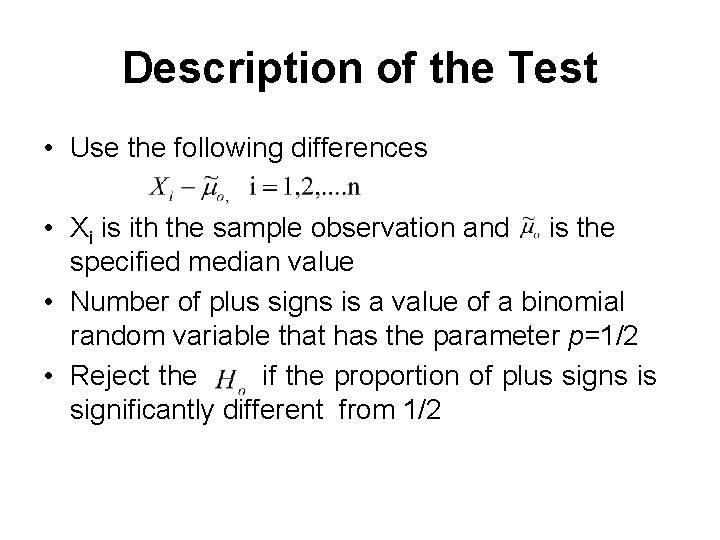
Description of the Test • Use the following differences • Xi is ith the sample observation and is the specified median value • Number of plus signs is a value of a binomial random variable that has the parameter p=1/2 • Reject the if the proportion of plus signs is significantly different from 1/2

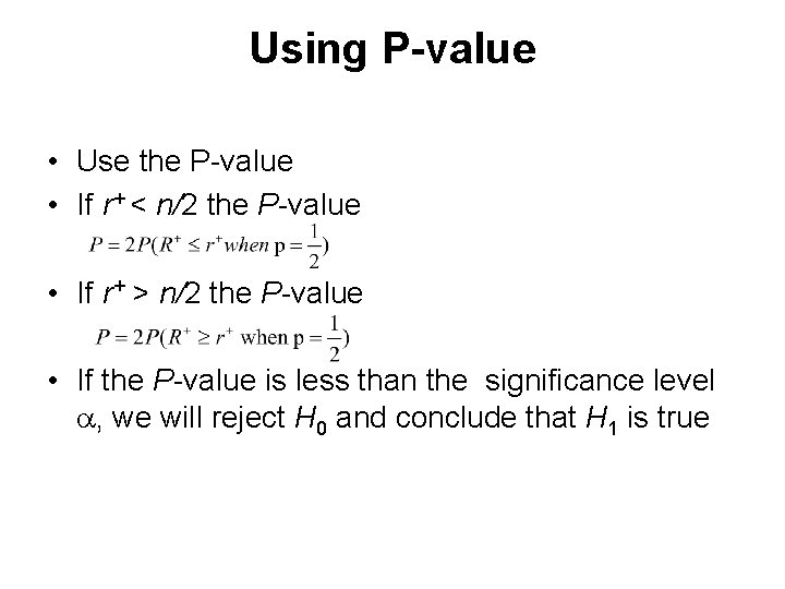
Using P-value • Use the P-value • If r+ < n/2 the P-value • If r+ > n/2 the P-value • If the P-value is less than the significance level , we will reject H 0 and conclude that H 1 is true

The Normal Approximation • Binomial distribution has well approximately a normal distribution when n >10 and p=0. 5 • Mean=np and the variance=np(1 -p) • Test statistics • Critical region can be chosen from the table of the standard normal distribution

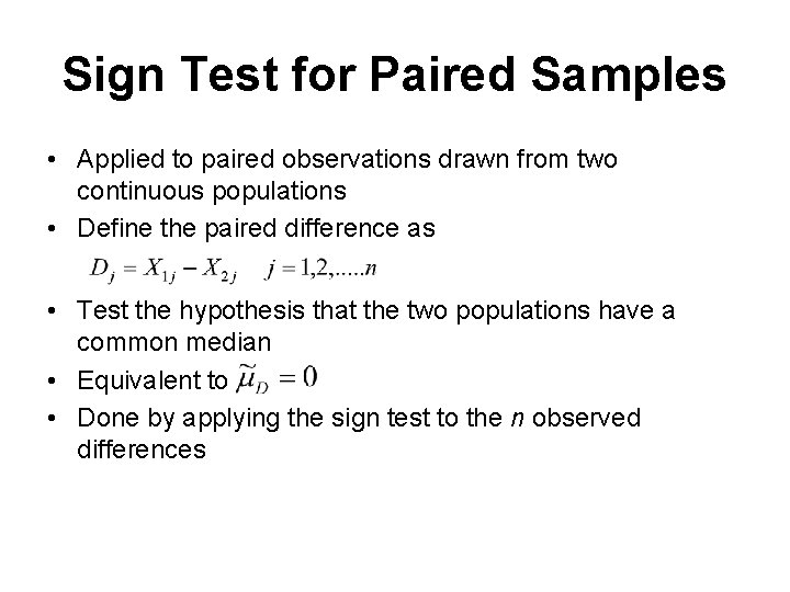
Sign Test for Paired Samples • Applied to paired observations drawn from two continuous populations • Define the paired difference as • Test the hypothesis that the two populations have a common median • Equivalent to • Done by applying the sign test to the n observed differences

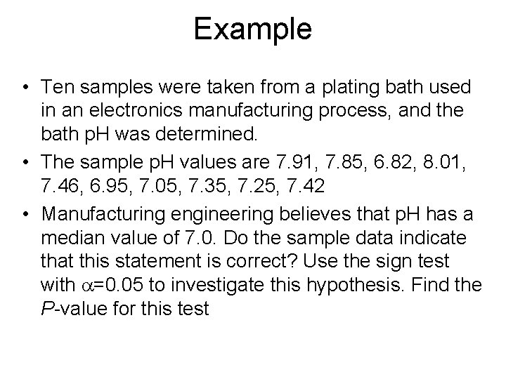
Example • Ten samples were taken from a plating bath used in an electronics manufacturing process, and the bath p. H was determined. • The sample p. H values are 7. 91, 7. 85, 6. 82, 8. 01, 7. 46, 6. 95, 7. 05, 7. 35, 7. 25, 7. 42 • Manufacturing engineering believes that p. H has a median value of 7. 0. Do the sample data indicate that this statement is correct? Use the sign test with =0. 05 to investigate this hypothesis. Find the P-value for this test

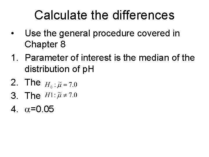
Calculate the differences • 1. 2. 3. 4. Use the general procedure covered in Chapter 8 Parameter of interest is the median of the distribution of p. H The =0. 05

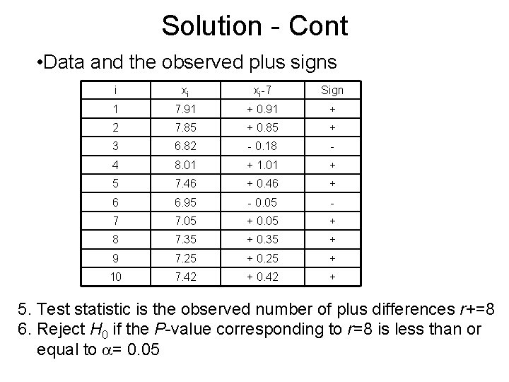
Solution - Cont • Data and the observed plus signs i xi xi-7 Sign 1 7. 91 + 0. 91 + 2 7. 85 + 0. 85 + 3 6. 82 - 0. 18 - 4 8. 01 + 1. 01 + 5 7. 46 + 0. 46 + 6 6. 95 - 0. 05 - 7 7. 05 + 0. 05 + 8 7. 35 + 0. 35 + 9 7. 25 + 0. 25 + 10 7. 42 + 0. 42 + 5. Test statistic is the observed number of plus differences r+=8 6. Reject H 0 if the P-value corresponding to r=8 is less than or equal to = 0. 05

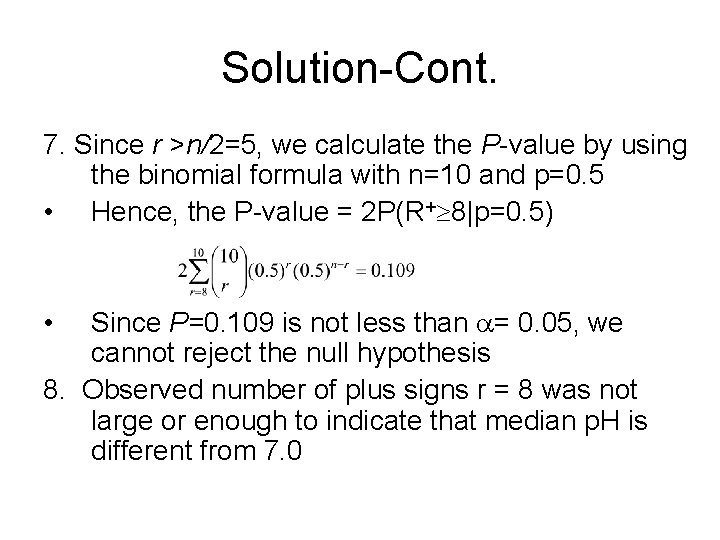
Solution-Cont. 7. Since r >n/2=5, we calculate the P-value by using the binomial formula with n=10 and p=0. 5 • Hence, the P-value = 2 P(R+ 8|p=0. 5) Since P=0. 109 is not less than = 0. 05, we cannot reject the null hypothesis 8. Observed number of plus signs r = 8 was not large or enough to indicate that median p. H is different from 7. 0 •

Using Table • Table of critical values for the sign test • Appendix Table VII is for two-sided and onesided alternative hypothesis • Let R=min (R+, R-) • Reject H 0 – If r-≤ critical value; if (>) used for H 1 – If r+≤ critical value; if (<) used for H 1 – If r≤ critical value; if (≠) used for H 1

Wilcoxon Signed-rank Test • Sign test uses only the plus and minus signs of the differences • Does not take into consideration the size or magnitude of these differences • Uses both direction (sign) and magnitude • In case of symmetric and continuous distributions • Test H 0 as µ=µ 0

Description of the Test • Compute the following quantities X i- 0 • Xi is ith the sample observation i and 0 is the specified median or mean value • Rank the absolute differences in ascending order • Give the ranks the signs • W+ be the sum of the positive ranks and W- be the sum of the negative ranks, and let W min(W+, W- ) • Table VIII contains critical values of W • Reject H 0 – If w-≤ critical value; if (>) used for H 1 – If w+≤ critical value; if (<) used for H 1 – If w≤ critical value; if (≠) used for H 1

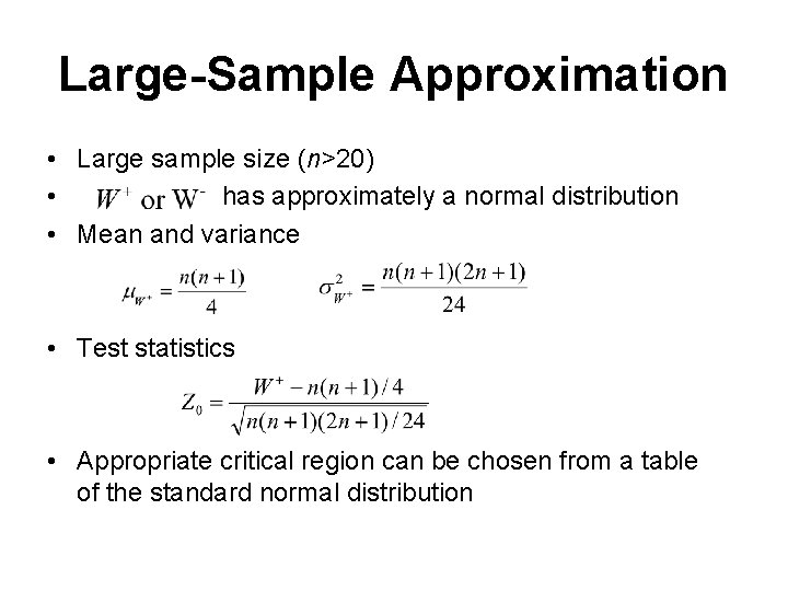
Large-Sample Approximation • Large sample size (n>20) • has approximately a normal distribution • Mean and variance • Test statistics • Appropriate critical region can be chosen from a table of the standard normal distribution

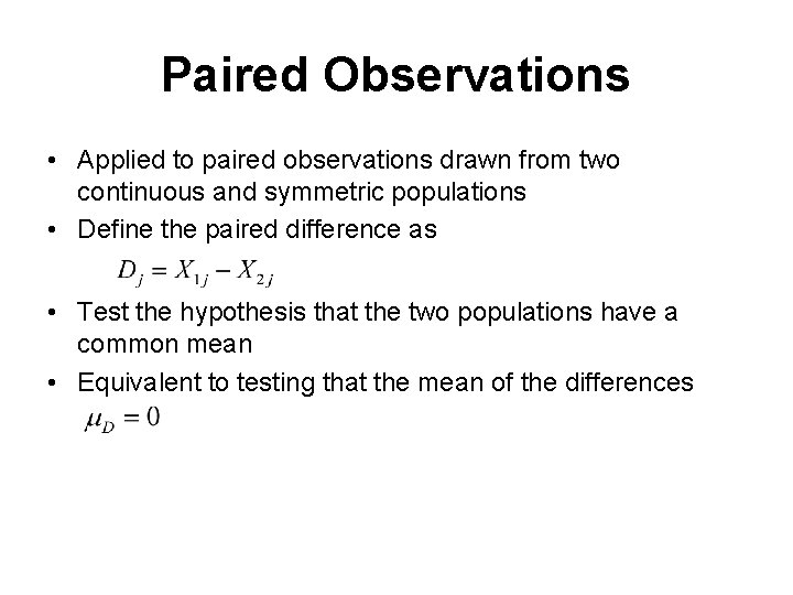
Paired Observations • Applied to paired observations drawn from two continuous and symmetric populations • Define the paired difference as • Test the hypothesis that the two populations have a common mean • Equivalent to testing that the mean of the differences

Description of the Test • Differences are first ranked in ascending order of their absolute values • Ranks are given the signs of the differences • Ties are assigned average ranks • W+ be the sum of the positive ranks and W- be the sum of the negative ranks, and let W min(W+, W- ) • Table VIII contains critical values of W • Reject H 0 – If w-≤ critical value; if (>) used for H 1 – If w+≤ critical value; if (<) used for H 1 – If w≤ critical value; if (≠) used for H 1

Example • Consider the data in the previous example and assume that the distribution of p. H is symmetric and continuous. • Use the Wilcoxon signed-rank test with =0. 05 to test the following hypothesis H 0: µ=7 vs. H 1: µ≠ 7

Solution 1. Parameter of interest is the mean of the p. H 2. H 0: µ=7 3. H 1: µ≠ 7 4. α=0. 05 5. Test statistic w=min (w+, w-) 6. Reject H 0 if w<w*0. 05=8 from Table VIII

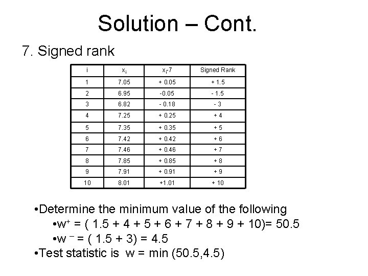
Solution – Cont. 7. Signed rank i xi xi-7 Signed Rank 1 7. 05 + 0. 05 + 1. 5 2 6. 95 -0. 05 - 1. 5 3 6. 82 - 0. 18 -3 4 7. 25 + 0. 25 +4 5 7. 35 + 0. 35 +5 6 7. 42 + 0. 42 +6 7 7. 46 + 0. 46 +7 8 7. 85 + 0. 85 +8 9 7. 91 + 0. 91 +9 10 8. 01 +1. 01 + 10 • Determine the minimum value of the following • w+ = ( 1. 5 + 4 + 5 + 6 + 7 + 8 + 9 + 10)= 50. 5 • w – = ( 1. 5 + 3) = 4. 5 • Test statistic is w = min (50. 5, 4. 5)

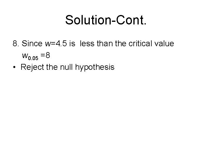
Solution-Cont. 8. Since w=4. 5 is less than the critical value w 0. 05 =8 • Reject the null hypothesis

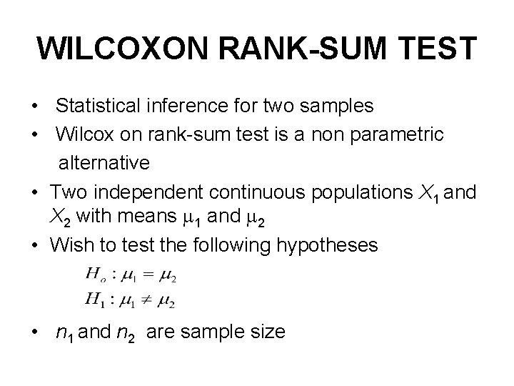
WILCOXON RANK-SUM TEST • Statistical inference for two samples • Wilcox on rank-sum test is a non parametric alternative • Two independent continuous populations X 1 and X 2 with means 1 and 2 • Wish to test the following hypotheses • n 1 and n 2 are sample size

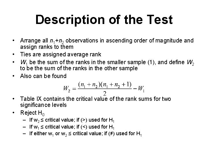
Description of the Test • Arrange all n 1+n 2 observations in ascending order of magnitude and assign ranks to them • Ties are assigned average rank • W 1 be the sum of the ranks in the smaller sample (1), and define W 2 to be the sum of the ranks in the other sample • Also can be found • Table IX contains the critical value of the rank sums for two significance levels • Reject H 0 – If w 2 ≤ critical value; if (>) used for H 1 – If w 1 ≤ critical value; if (<) used for H 1 – If either w 1 or w 2 ≤ critical value; if (≠) used for H 1

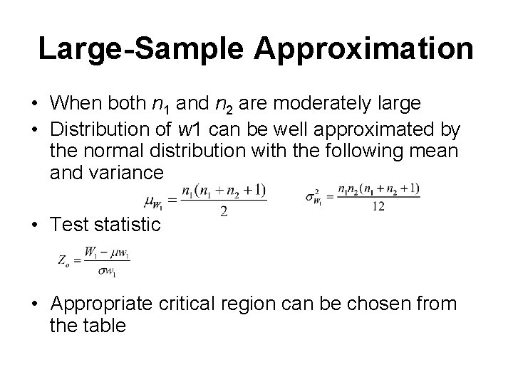
Large-Sample Approximation • When both n 1 and n 2 are moderately large • Distribution of w 1 can be well approximated by the normal distribution with the following mean and variance • Test statistic • Appropriate critical region can be chosen from the table

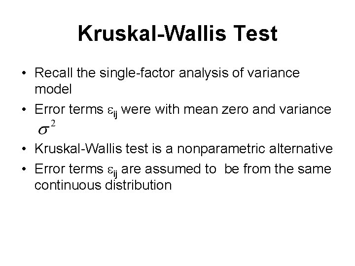
Kruskal-Wallis Test • Recall the single-factor analysis of variance model • Error terms ij were with mean zero and variance • Kruskal-Wallis test is a nonparametric alternative • Error terms ij are assumed to be from the same continuous distribution

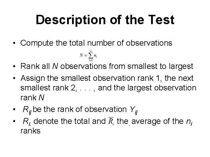
Description of the Test • Compute the total number of observations • Rank all N observations from smallest to largest • Assign the smallest observation rank 1, the next smallest rank 2, . . . , and the largest observation rank N • Rij be the rank of observation Yij • Ri. denote the total and the. average of the ni ranks

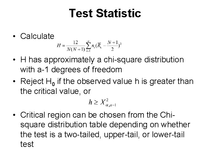
Test Statistic • Calculate • H has approximately a chi-square distribution with a-1 degrees of freedom • Reject H 0 if the observed value h is greater than the critical value, or • Critical region can be chosen from the Chisquare distribution table depending on whether the test is a two-tailed, upper-tail, or lower-tail test

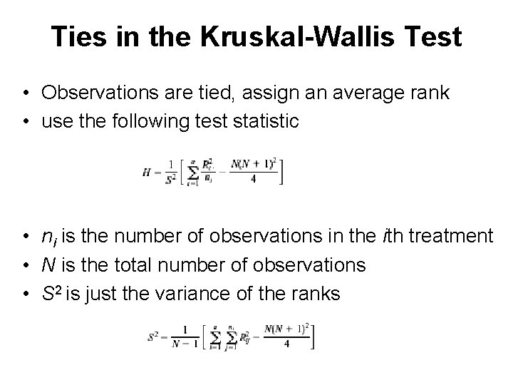
Ties in the Kruskal-Wallis Test • Observations are tied, assign an average rank • use the following test statistic • ni is the number of observations in the ith treatment • N is the total number of observations • S 2 is just the variance of the ranks

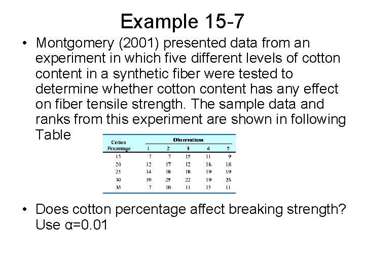
Example 15 -7 • Montgomery (2001) presented data from an experiment in which five different levels of cotton content in a synthetic fiber were tested to determine whether cotton content has any effect on fiber tensile strength. The sample data and ranks from this experiment are shown in following Table • Does cotton percentage affect breaking strength? Use α=0. 01

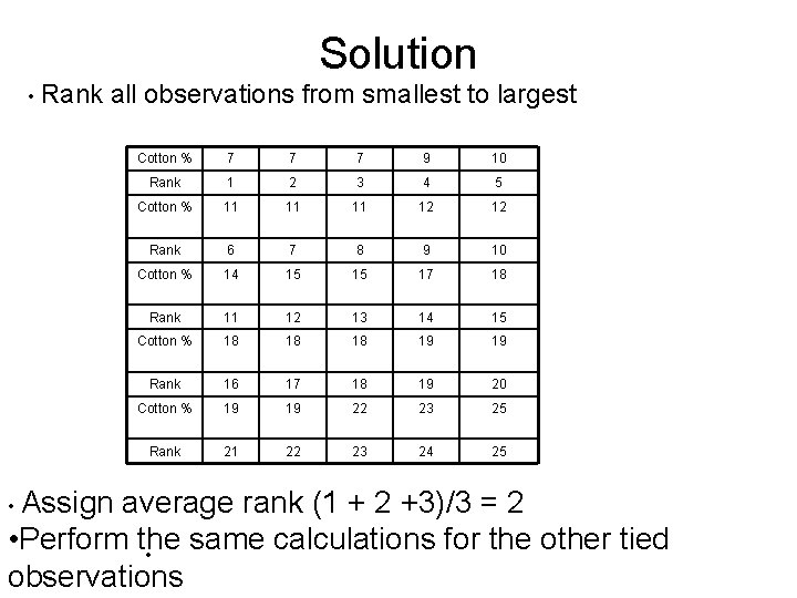
Solution • Rank all observations from smallest to largest • Assign Cotton % 7 7 7 9 10 Rank 1 2 3 4 5 Cotton % 11 11 11 12 12 Rank 6 7 8 9 10 Cotton % 14 15 15 17 18 Rank 11 12 13 14 15 Cotton % 18 18 18 19 19 Rank 16 17 18 19 20 Cotton % 19 19 22 23 25 Rank 21 22 23 24 25 average rank (1 + 2 +3)/3 = 2 • Perform the same calculations for the other tied • observations

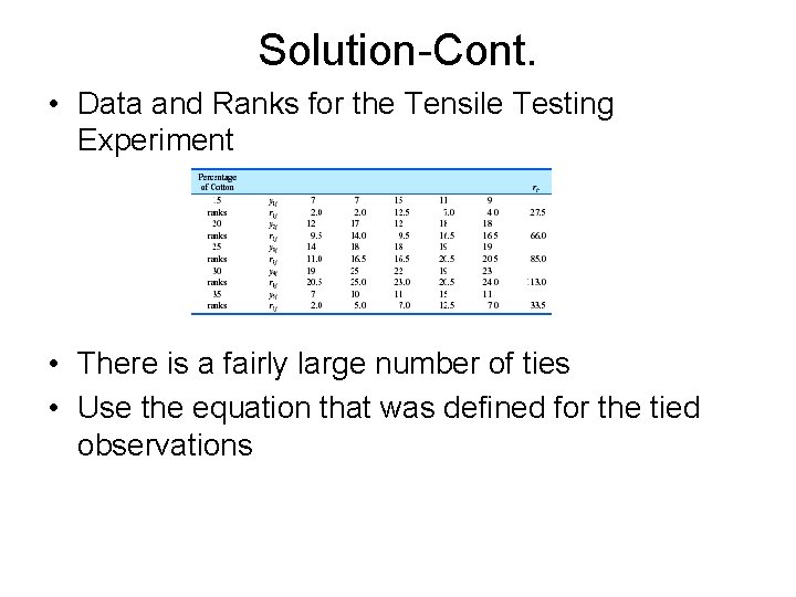
Solution-Cont. • Data and Ranks for the Tensile Testing Experiment • There is a fairly large number of ties • Use the equation that was defined for the tied observations

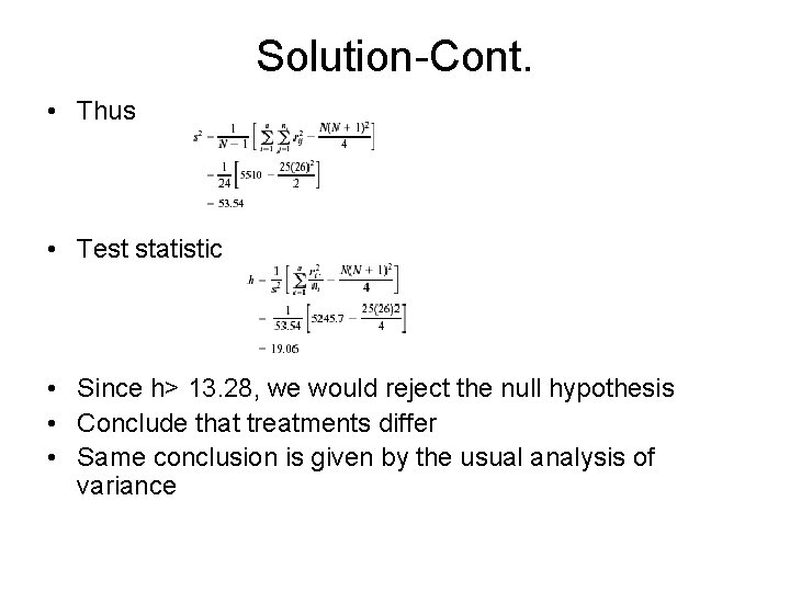
Solution-Cont. • Thus • Test statistic • Since h> 13. 28, we would reject the null hypothesis • Conclude that treatments differ • Same conclusion is given by the usual analysis of variance

Next Agenda • Introduces statistical quality control • Fundamentals of statistical process control