Chapter 15 Decisions Under Risk and Uncertainty Mc

Chapter 15: Decisions Under Risk and Uncertainty Mc. Graw-Hill/Irwin Copyright © 2011 by the Mc. Graw-Hill Companies, Inc. All rights reserved.

In business we are forced to make decisions involving risk—that is, where the consequences of any action we take is uncertain due to unforeseeable events. Where do we begin? 15 -2

Risk vs. Uncertainty • Risk • Must make a decision for which the outcome is not known with certainty • Can list all possible outcomes & assign probabilities to the outcomes • Uncertainty • Cannot list all possible outcomes • Cannot assign probabilities to the outcomes 15 -3

The game of roulette is subject to risk. The return on investment in R & D is subject to uncertainty. 15 -4

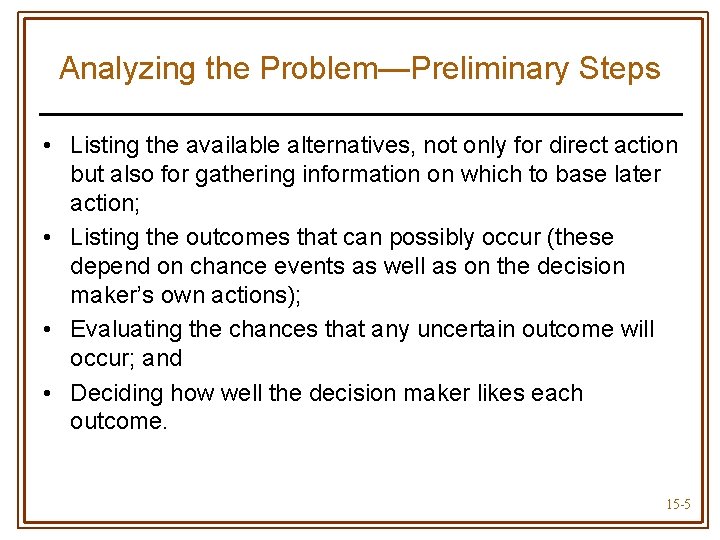
Analyzing the Problem—Preliminary Steps • Listing the available alternatives, not only for direct action but also for gathering information on which to base later action; • Listing the outcomes that can possibly occur (these depend on chance events as well as on the decision maker’s own actions); • Evaluating the chances that any uncertain outcome will occur; and • Deciding how well the decision maker likes each outcome. 15 -5

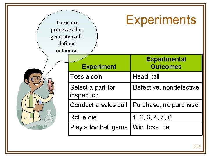
These are processes that generate welldefined outcomes Experiments Experimental Outcomes Toss a coin Head, tail Select a part for inspection Defective, nondefective Conduct a sales call Purchase, no purchase Roll a die 1, 2, 3, 4, 5, 6 Play a football game Win, lose, tie 15 -6

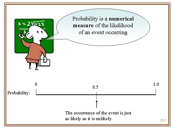
Probability is a numerical measure of the likelihood of an event occurring 0 0. 5 1. 0 Probability: The occurrence of the event is just as likely as it is unlikely 15 -7

Unfortunately, business experiments are rarely repeatable. We cannot introduce a new product 1, 000 times and measure the frequency with which it succeeds—can we? 15 -8

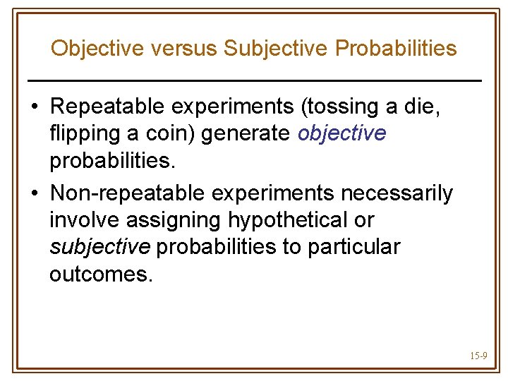
Objective versus Subjective Probabilities • Repeatable experiments (tossing a die, flipping a coin) generate objective probabilities. • Non-repeatable experiments necessarily involve assigning hypothetical or subjective probabilities to particular outcomes. 15 -9

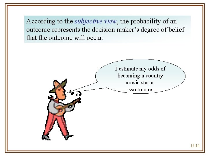
According to the subjective view, the probability of an outcome represents the decision maker’s degree of belief that the outcome will occur. I estimate my odds of becoming a country music star at two to one. 15 -10

Measuring Risk with Probability Distributions • Table or graph showing all possible outcomes/payoffs for a decision & the probability each outcome will occur • To measure risk associated with a decision • Examine statistical characteristics of the probability distribution of outcomes for the decision 15 -11

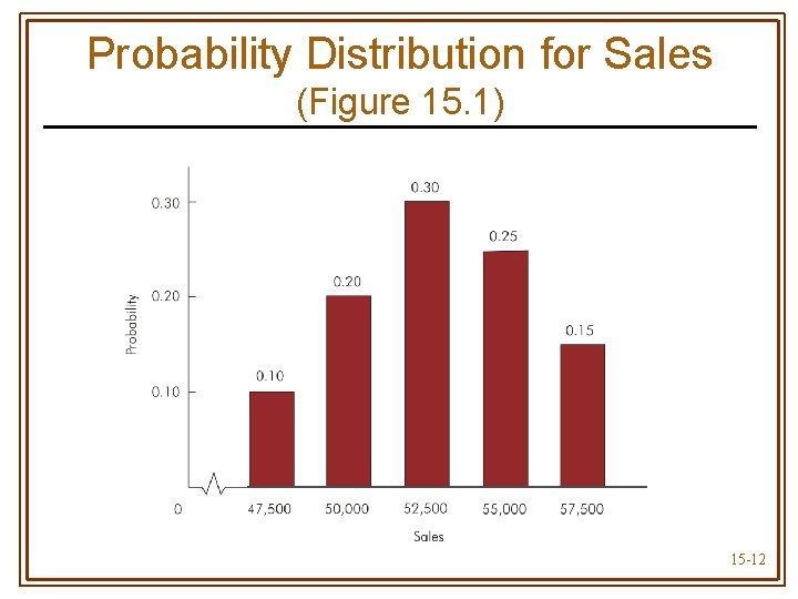
Probability Distribution for Sales (Figure 15. 1) 15 -12

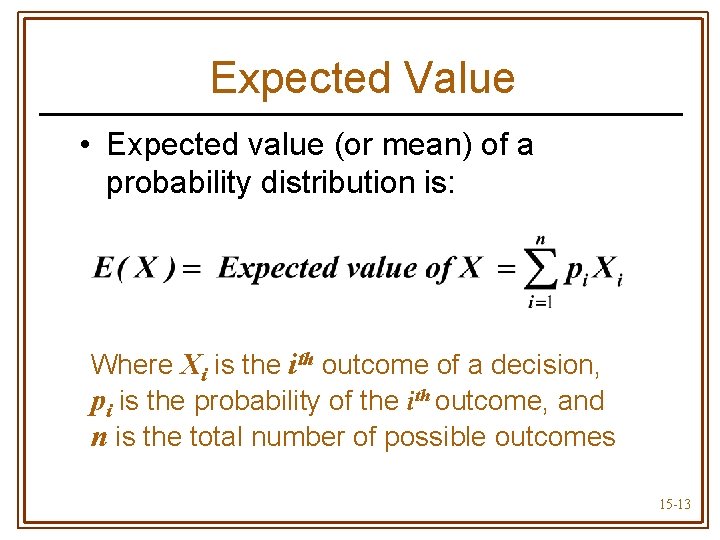
Expected Value • Expected value (or mean) of a probability distribution is: Where Xi is the ith outcome of a decision, pi is the probability of the ith outcome, and n is the total number of possible outcomes 15 -13

Expected Value • Does not give actual value of the random outcome • Indicates “average” value of the outcomes if the risky decision were to be repeated a large number of times 15 -14

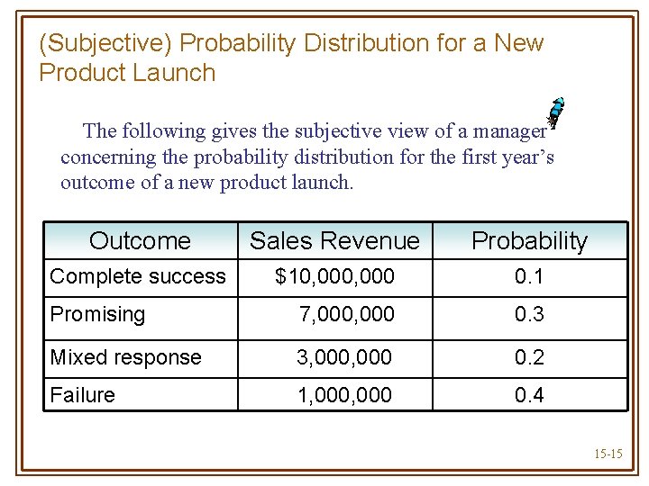
(Subjective) Probability Distribution for a New Product Launch The following gives the subjective view of a manager concerning the probability distribution for the first year’s outcome of a new product launch. Outcome Sales Revenue Probability Complete success $10, 000 0. 1 Promising 7, 000 0. 3 Mixed response 3, 000 0. 2 Failure 1, 000 0. 4 15 -15

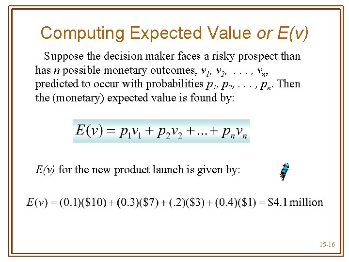
Computing Expected Value or E(v) Suppose the decision maker faces a risky prospect than has n possible monetary outcomes, v 1, v 2, . . . , vn, predicted to occur with probabilities p 1, p 2, . . . , pn. Then the (monetary) expected value is found by: E(v) for the new product launch is given by: 15 -16

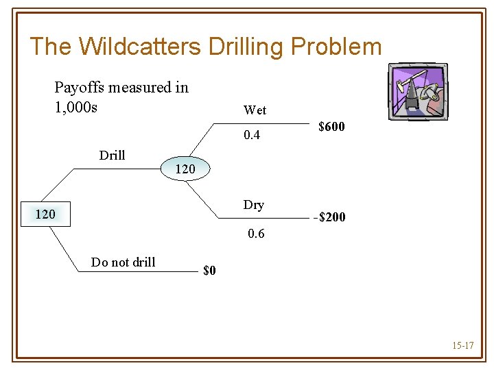
The Wildcatters Drilling Problem Payoffs measured in 1, 000 s Wet 0. 4 Drill $600 120 Dry 120 -$200 0. 6 Do not drill $0 15 -17

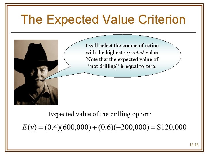
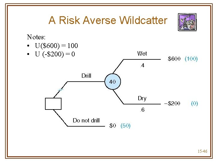
The Expected Value Criterion I will select the course of action with the highest expected value. Note that the expected value of “not drilling” is equal to zero. Expected value of the drilling option: 15 -18

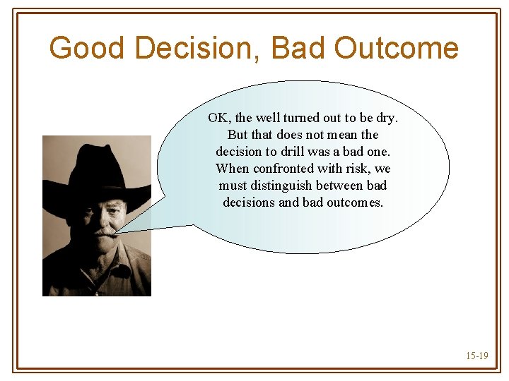
Good Decision, Bad Outcome OK, the well turned out to be dry. But that does not mean the decision to drill was a bad one. When confronted with risk, we must distinguish between bad decisions and bad outcomes. 15 -19

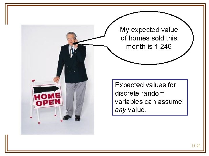
My expected value of homes sold this month is 1. 246 Expected values for discrete random variables can assume any value. 15 -20

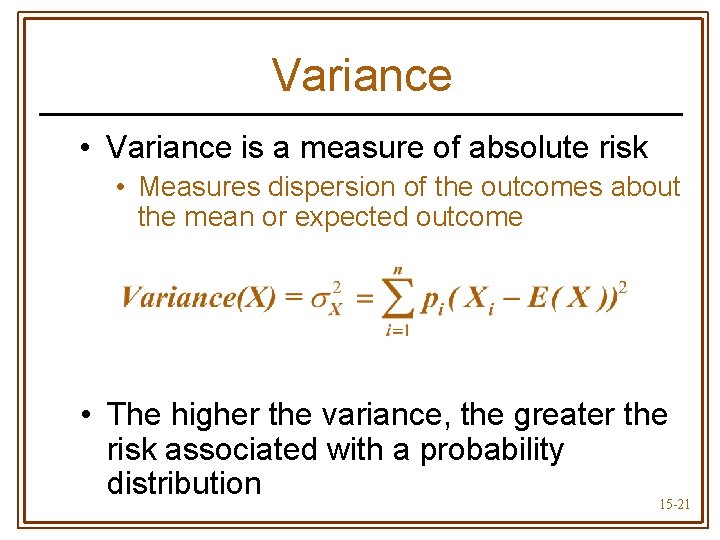
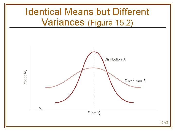
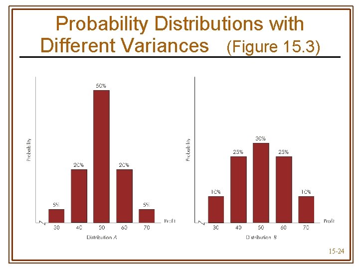
Variance • Variance is a measure of absolute risk • Measures dispersion of the outcomes about the mean or expected outcome • The higher the variance, the greater the risk associated with a probability distribution 15 -21

Identical Means but Different Variances (Figure 15. 2) 15 -22

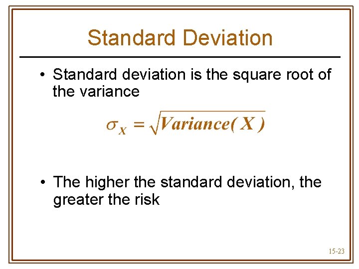
Standard Deviation • Standard deviation is the square root of the variance • The higher the standard deviation, the greater the risk 15 -23

Probability Distributions with Different Variances (Figure 15. 3) 15 -24

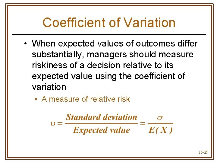
Coefficient of Variation • When expected values of outcomes differ substantially, managers should measure riskiness of a decision relative to its expected value using the coefficient of variation • A measure of relative risk 15 -25

Decisions Under Risk • No single decision rule guarantees profits will actually be maximized • Decision rules do not eliminate risk • Provide a method to systematically include risk in the decision making process 15 -26

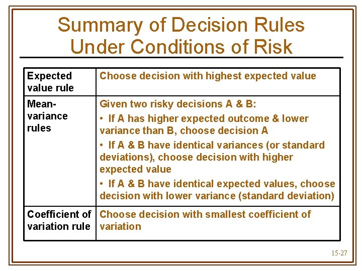
Summary of Decision Rules Under Conditions of Risk Expected value rule Choose decision with highest expected value Meanvariance rules Given two risky decisions A & B: • If A has higher expected outcome & lower variance than B, choose decision A • If A & B have identical variances (or standard deviations), choose decision with higher expected value • If A & B have identical expected values, choose decision with lower variance (standard deviation) Coefficient of Choose decision with smallest coefficient of variation rule variation 15 -27

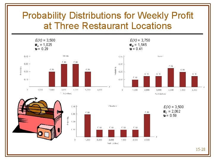
Probability Distributions for Weekly Profit at Three Restaurant Locations E(X) = 3, 500 A = 1, 025 = 0. 29 E(X) = 3, 750 B = 1, 545 = 0. 41 E(X) = 3, 500 C = 2, 062 = 0. 59 15 -28

Which Rule is Best? • For a repeated decision, with identical probabilities each time • Expected value rule is most reliable to maximizing (expected) profit • Average return of a given risky course of action repeated many times approaches the expected value of that action 15 -29

Which Rule is Best? • For a one-time decision under risk • No repetitions to “average out” a bad outcome • No best rule to follow • Rules should be used to help analyze & guide decision making process • As much art as science 15 -30

Expected Utility Theory • Actual decisions made depend on the willingness to accept risk • Expected utility theory allows for different attitudes toward risk-taking in decision making • Managers are assumed to derive utility from earning profits 15 -31

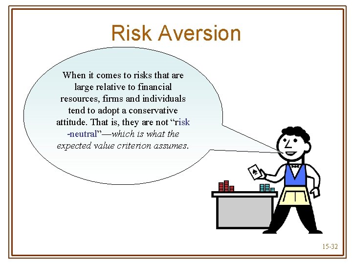
Risk Aversion When it comes to risks that are large relative to financial resources, firms and individuals tend to adopt a conservative attitude. That is, they are not “risk -neutral”—which is what the expected value criterion assumes. 15 -32

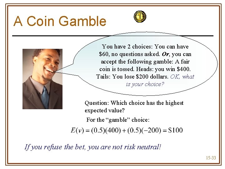
A Coin Gamble You have 2 choices: You can have $60, no questions asked. Or, you can accept the following gamble: A fair coin is tossed. Heads: you win $400. Tails: You lose $200 dollars. OK, what is your choice? Question: Which choice has the highest expected value? For the “gamble” choice: If you refuse the bet, you are not risk neutral! 15 -33

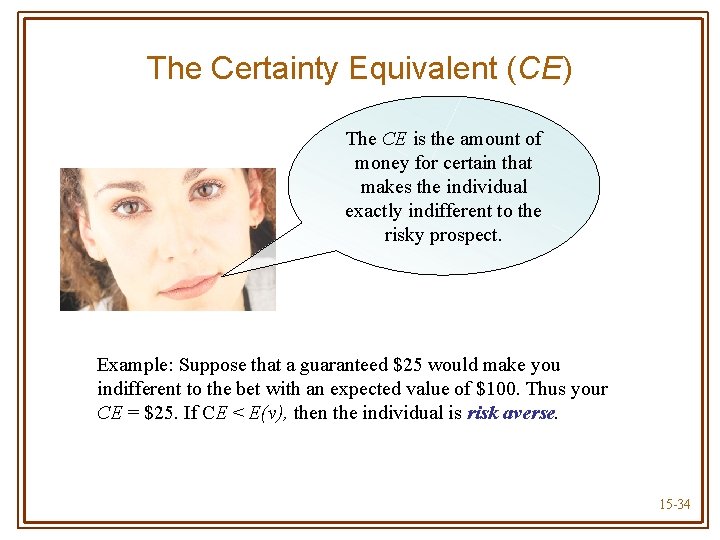
The Certainty Equivalent (CE) The CE is the amount of money for certain that makes the individual exactly indifferent to the risky prospect. Example: Suppose that a guaranteed $25 would make you indifferent to the bet with an expected value of $100. Thus your CE = $25. If CE < E(v), then the individual is risk averse. 15 -34

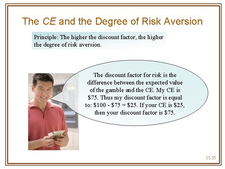
The CE and the Degree of Risk Aversion Principle: The higher the discount factor, the higher the degree of risk aversion. The discount factor for risk is the difference between the expected value of the gamble and the CE. My CE is $75. Thus my discount factor is equal to: $100 - $75 = $25. If your CE is $25, then your discount factor is $75. 15 -35

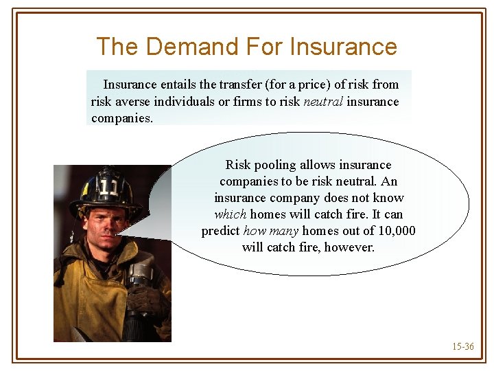
The Demand For Insurance entails the transfer (for a price) of risk from risk averse individuals or firms to risk neutral insurance companies. Risk pooling allows insurance companies to be risk neutral. An insurance company does not know which homes will catch fire. It can predict how many homes out of 10, 000 will catch fire, however. 15 -36

Expected Utility This is a similar decision making process to expected value—with one big difference. In contrast to the risk neutral manager, who averages monetary values at each step, the risk averse manager averages expected utilities associated with monetary values. 15 -37

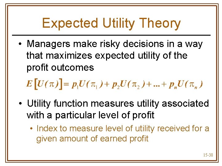
Expected Utility Theory • Managers make risky decisions in a way that maximizes expected utility of the profit outcomes • Utility function measures utility associated with a particular level of profit • Index to measure level of utility received for a given amount of earned profit 15 -38

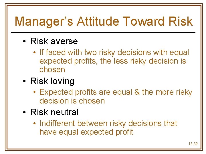
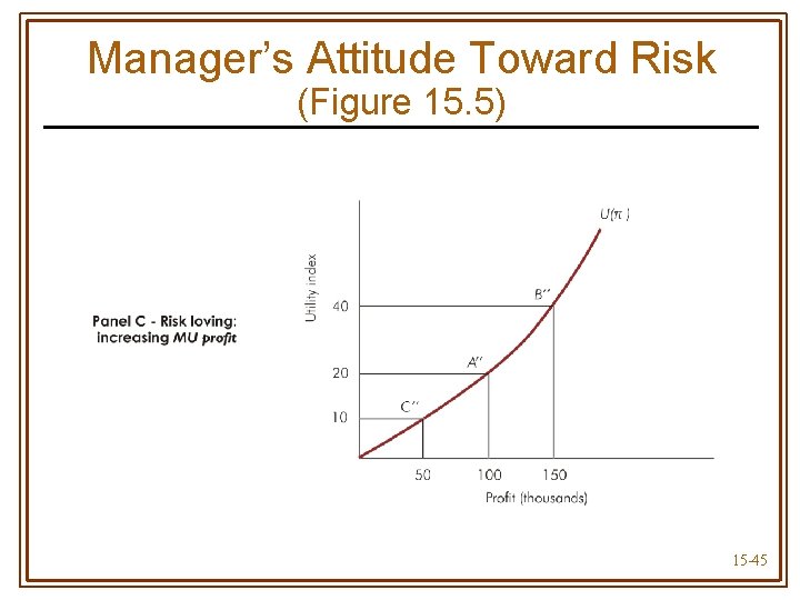
Manager’s Attitude Toward Risk • Risk averse • If faced with two risky decisions with equal expected profits, the less risky decision is chosen • Risk loving • Expected profits are equal & the more risky decision is chosen • Risk neutral • Indifferent between risky decisions that have equal expected profit 15 -39

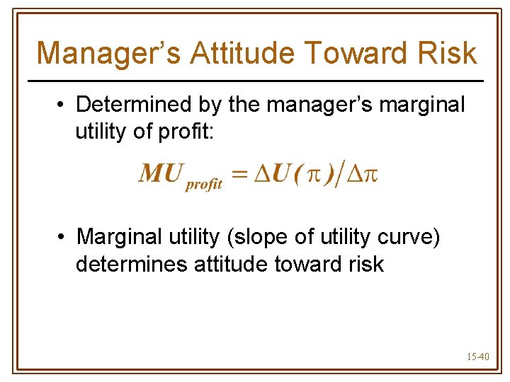
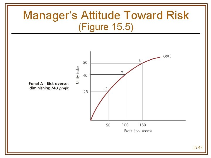
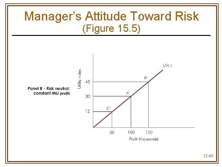
Manager’s Attitude Toward Risk • Determined by the manager’s marginal utility of profit: • Marginal utility (slope of utility curve) determines attitude toward risk 15 -40

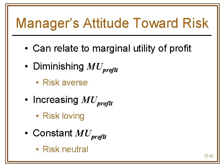
Manager’s Attitude Toward Risk • Can relate to marginal utility of profit • Diminishing MUprofit • Risk averse • Increasing MUprofit • Risk loving • Constant MUprofit • Risk neutral 15 -41

Expected Utility of Profits • According to expected utility theory, decisions are made to maximize the manager’s expected utility of profits • Such decisions reflect risk-taking attitude • Generally differ from those reached by decision rules that do not consider risk • For a risk-neutral manager, decisions are identical under maximization of expected utility or maximization of expected profit 15 -42

Manager’s Attitude Toward Risk (Figure 15. 5) 15 -43

Manager’s Attitude Toward Risk (Figure 15. 5) 15 -44

Manager’s Attitude Toward Risk (Figure 15. 5) 15 -45

A Risk Averse Wildcatter Notes: • U($600) = 100 • U (-$200) = 0 15 -46

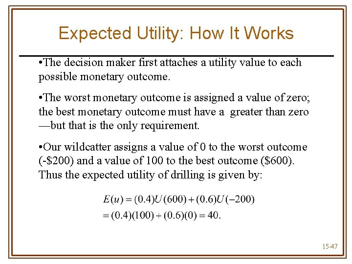
Expected Utility: How It Works • The decision maker first attaches a utility value to each possible monetary outcome. • The worst monetary outcome is assigned a value of zero; the best monetary outcome must have a greater than zero —but that is the only requirement. • Our wildcatter assigns a value of 0 to the worst outcome (-$200) and a value of 100 to the best outcome ($600). Thus the expected utility of drilling is given by: 15 -47

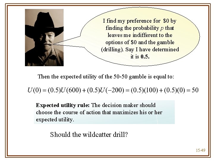
Expected Utility: How It Works-Continued Now I must compare the expected utility of drilling with the expected utility of not drilling—that is U(0). How do I find that? Principle: To find U(0), compare $0 for certain with a gamble offering $600 thousand (with probability p) and $200 thousand (with probability 1 – p). The wildcatter finds his preference for $0 by finding the probability p that leaves him indifferent to the options of $0 and the gamble (drilling). 15 -48

I find my preference for $0 by finding the probability p that leaves me indifferent to the options of $0 and the gamble (drilling). Say I have determined it is 0. 5. Then the expected utility of the 50 -50 gamble is equal to: Expected utility rule: The decision maker should choose the course of action that maximizes his or her expected utility. Should the wildcatter drill? 15 -49

15 -50

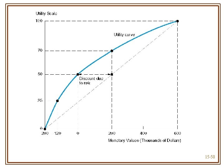
Notes on Preceding Figure • The utility curve gives us the “certainty equivalent” of a bet with a given expected value. • The CE of a bet with an expected value of $200 thousand is $0. That is, the certainty of obtaining $0 and a bet with an expected value of $200 thousand have the same expected utility (50). • A concave utility curve means the decision maker is risk averse—that is, there is a discount due to risk equal to E(v) – CE ($200 thousand in the example above). • A risk-neutral decision maker is guided by expected value—there is no discount for risk so that the utility curve is linear. • A risk lover has a convex utility curve. 15 -51