Chapter 15 Control Methods Control is the heart

Chapter 15 Control Methods

Control is the heart of Six Sigma Customers are demanding higher levels of product quality at a lower cost, improved responsiveness, and added value. + Producers must struggle to satisfy technical, performance, schedule, and cost expectations of the customer. = Drive the need for control methods used in Six Sigma & TQM Do it right the first time Eliminate product variation ↓ Delivery of offerings, which are defect free at a min. cycle time

Six Sigma initiatives to reduce variation In the past, the pursuit of quality was more a philosophy than an art or science… these tools can change that. Design • Design to standard parts • Design to standard materials • Robust design • Design for assembly • Design for reliability • Design for simplicity Process • Short-cycle manufacturing • Process characterization • Process standardization • Statistical process control Material and Components • Part standardization • Transaction(s) standardization • Supplier statistical process control (SPC) • Supplier certification • Material requirements planning

Poka-Yoke • Japanese for mistake proofing – Poka (inadvertent error) – Yokeru (avoidance) • Design and implementation of actions to prevent errors, mistakes, or defects in our everyday activities and processes. • Errors should not be considered inevitable. Any error type can be reduced considerably, if not eliminated altogether. http: //www. youtube. com/watch? v=Nrnlo. Z 12 KGs

Common types of mistakes • • • Incorrect processing Work pieces placed incorrectly Missing parts Wrong blue print or instructions Wrong piece processed Operation skipped or omitted Improper adjustment Equipment not set up properly Process improperly supersized Use of the wrong tool

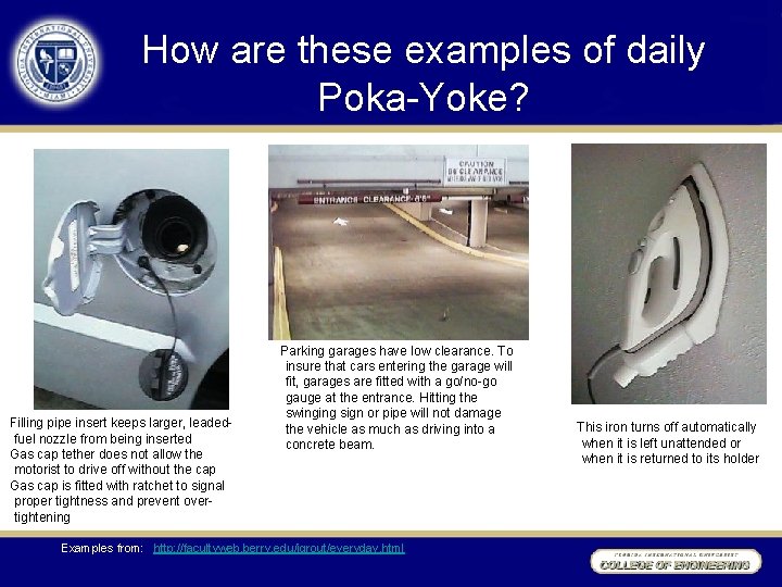
How are these examples of daily Poka-Yoke? Filling pipe insert keeps larger, leadedfuel nozzle from being inserted Gas cap tether does not allow the motorist to drive off without the cap Gas cap is fitted with ratchet to signal proper tightness and prevent overtightening Parking garages have low clearance. To insure that cars entering the garage will fit, garages are fitted with a go/no-go gauge at the entrance. Hitting the swinging sign or pipe will not damage the vehicle as much as driving into a concrete beam. Examples from: http: //facultyweb. berry. edu/jgrout/everyday. html This iron turns off automatically when it is left unattended or when it is returned to its holder

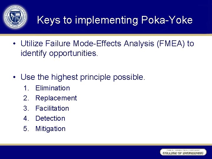
Keys to implementing Poka-Yoke • Utilize Failure Mode-Effects Analysis (FMEA) to identify opportunities. • Use the highest principle possible. 1. 2. 3. 4. 5. Elimination Replacement Facilitation Detection Mitigation

Statistical Process Control (SPC) • SPC is a method of analyzing data over time and using the result of the analysis to solve manufacturing and processing problems – Can be applied to almost anything that can be expressed with numbers of data. • Control = to keep something within boundaries • Process = any set of conditions or causes, which work together to produce an output or result. • Process is a sequence of activities characterized by: 1. 2. 3. 4. Measureable inputs Value-added (VA) activities Measureable Outputs Repeatability

Statistical Control • A process is within statistical control when the process contains only natural, chance variation. – Only when a process is statistically stable can it be treated as a population with constant mean, standard deviation, and distribution. • A process control system is a feedback four element system: 1. 2. 3. 4. The Process Information about Performance Action on the Process Actions on the Output

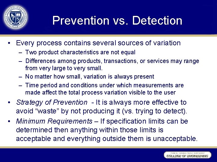
Prevention vs. Detection • Every process contains several sources of variation – Two product characteristics are not equal – Differences among products, transactions, or services may range from very large to very small. – No matter how small, variation is always present – Time period and conditions under which measurements are made affect the total process variation visible to the user • Strategy of Prevention - It is always more effective to avoid “waste” by not producing it (vs. trying to detect). • Minimum Requirements – If specification limits can be determined then anything within those limits is acceptable and everything outside them is unacceptable.

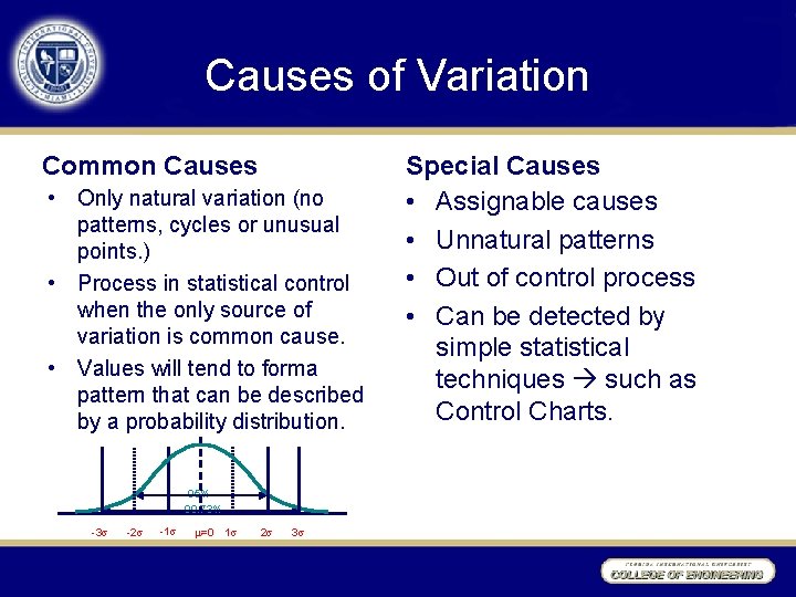
Causes of Variation Common Causes • Only natural variation (no patterns, cycles or unusual points. ) • Process in statistical control when the only source of variation is common cause. • Values will tend to forma pattern that can be described by a probability distribution. 95% 99. 73% -3 -2 -1 =0 1 2 3 Special Causes • Assignable causes • Unnatural patterns • Out of control process • Can be detected by simple statistical techniques such as Control Charts.

Continuous Statistical Process Control (SPC) Tools • Purposes of Control Charts 1. Control a CTP characteristic (statistical process control - SPC) 2. Used to monitor a CTQ, CTC or CTD characteristic (Statistical process monitoring-SPM) 3. Used as diagnostic tools for any CT Characteristic.

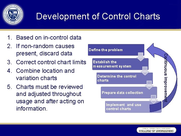
Development of Control Charts Define the problem Establish the measurement system Determine the control charts Prepare data collection Implement and use control charts Continuous Improvement 1. Based on in-control data 2. If non-random causes present, discard data 3. Correct control chart limits 4. Combine location and variation charts 5. Charts must be reviewed and adjusted throughout usage and after acting on information.

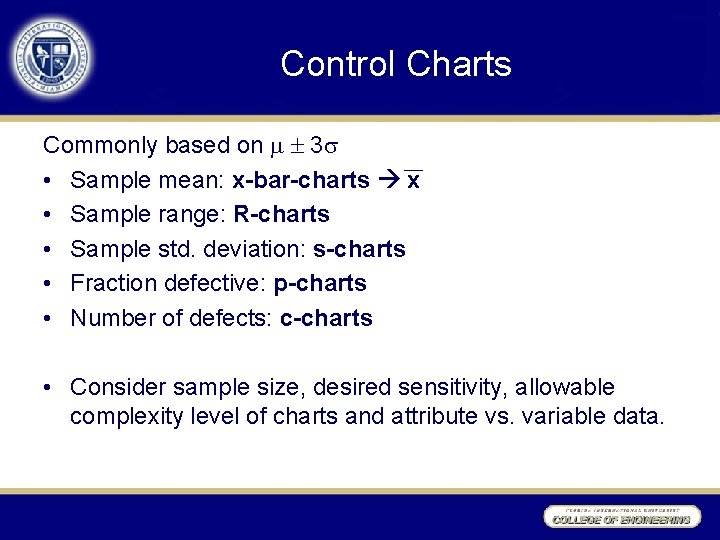
Control Charts Commonly based on 3 • Sample mean: x-bar-charts x • Sample range: R-charts • Sample std. deviation: s-charts • Fraction defective: p-charts • Number of defects: c-charts • Consider sample size, desired sensitivity, allowable complexity level of charts and attribute vs. variable data.

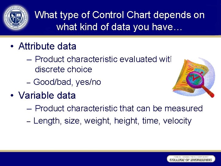
What type of Control Chart depends on what kind of data you have… • Attribute data – Product characteristic evaluated with a discrete choice – Good/bad, yes/no • Variable data – Product characteristic that can be measured – Length, size, weight, height, time, velocity

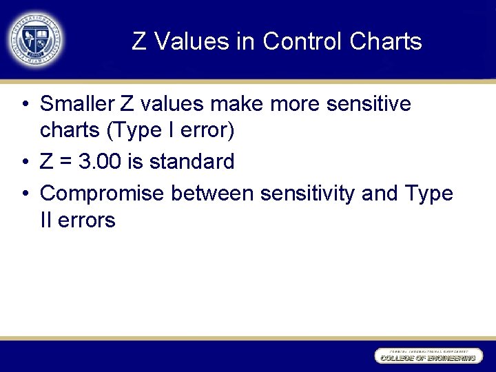
Z Values in Control Charts • Smaller Z values make more sensitive charts (Type I error) • Z = 3. 00 is standard • Compromise between sensitivity and Type II errors

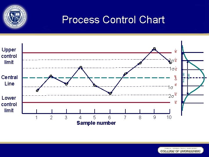
Process Control Chart -3 Upper control limit -2 2 3 1 2 3 4 5 6 Sample number 7 8 9 10 95% 2 2 Lower control limit 99. 73% 1 =0 1 Central Line -1 1

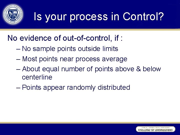
Is your process in Control? No evidence of out-of-control, if : – No sample points outside limits – Most points near process average – About equal number of points above & below centerline – Points appear randomly distributed

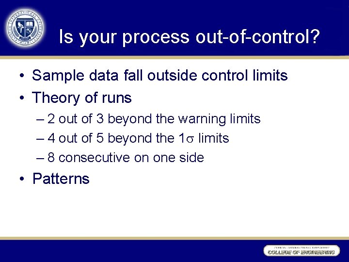
Is your process out-of-control? • Sample data fall outside control limits • Theory of runs – 2 out of 3 beyond the warning limits – 4 out of 5 beyond the 1 limits – 8 consecutive on one side • Patterns

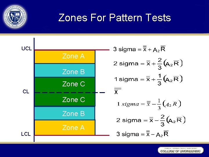
Zones For Pattern Tests UCL Zone A Zone B Zone C CL Zone C Zone B LCL Zone A

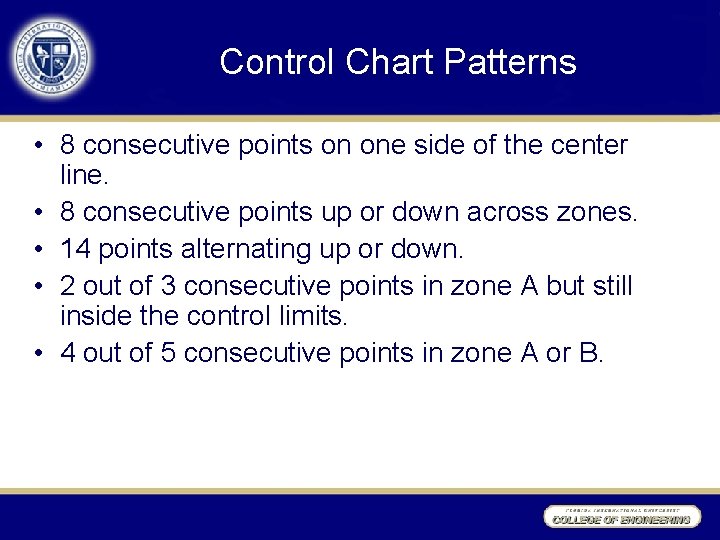
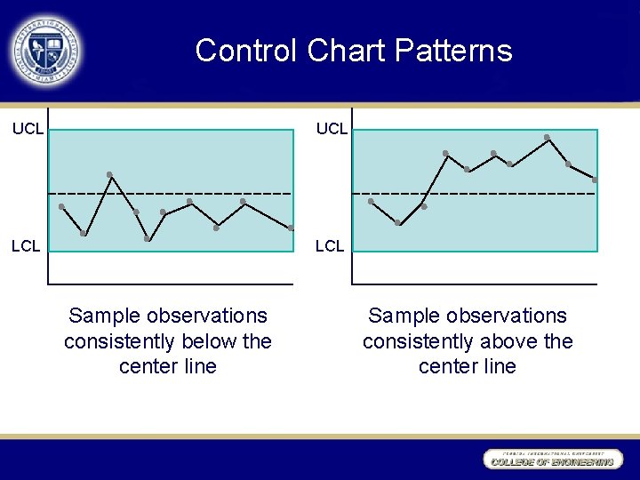
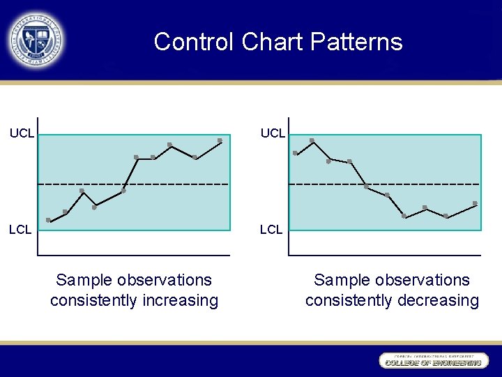
Control Chart Patterns • 8 consecutive points on one side of the center line. • 8 consecutive points up or down across zones. • 14 points alternating up or down. • 2 out of 3 consecutive points in zone A but still inside the control limits. • 4 out of 5 consecutive points in zone A or B.

Control Chart Patterns UCL LCL Sample observations consistently below the center line Sample observations consistently above the center line

Control Chart Patterns UCL LCL Sample observations consistently increasing Sample observations consistently decreasing

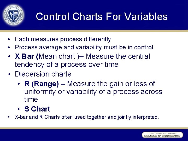
Control Charts For Variables • Each measures process differently • Process average and variability must be in control • X Bar (Mean chart )– Measure the central tendency of a process over time • Dispersion charts • R (Range) – Measure the gain or loss of uniformity or variability of a process across time • S Chart • X-bar and R Charts often used together and jointly interpreted.

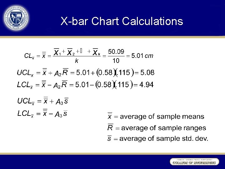
X-bar Chart Calculations

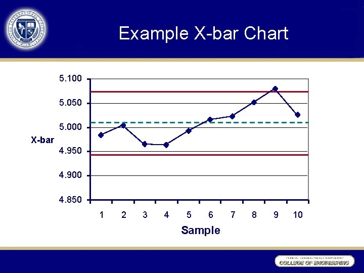
Example X-bar Chart 5. 100 5. 050 5. 000 X-bar 4. 950 4. 900 4. 850 1 2 3 4 5 6 Sample 7 8 9 10

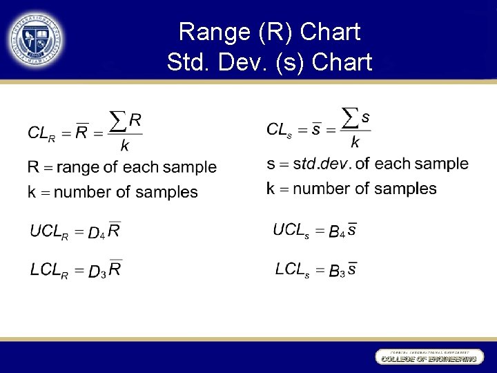
Range (R) Chart Std. Dev. (s) Chart

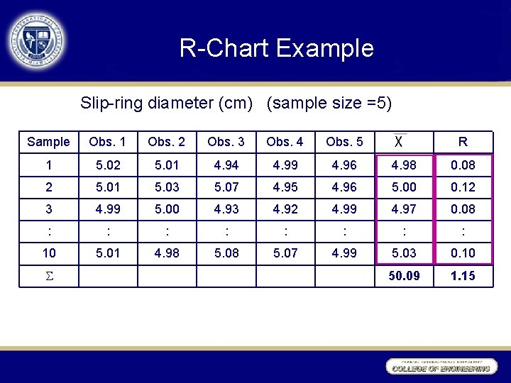
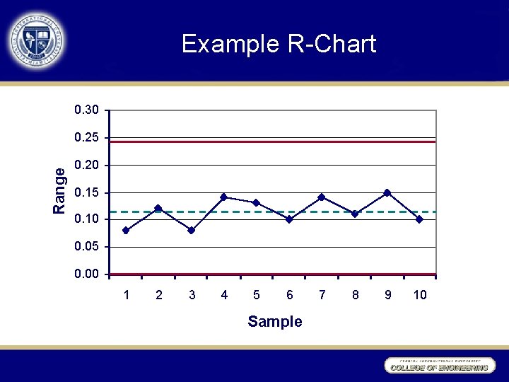
R-Chart Example Slip-ring diameter (cm) (sample size =5) Sample Obs. 1 Obs. 2 Obs. 3 Obs. 4 Obs. 5 1 5. 02 5. 01 4. 94 4. 99 4. 96 4. 98 0. 08 2 5. 01 5. 03 5. 07 4. 95 4. 96 5. 00 0. 12 3 4. 99 5. 00 4. 93 4. 92 4. 99 4. 97 0. 08 : : 10 5. 01 4. 98 5. 07 4. 99 5. 03 0. 10 50. 09 1. 15 R

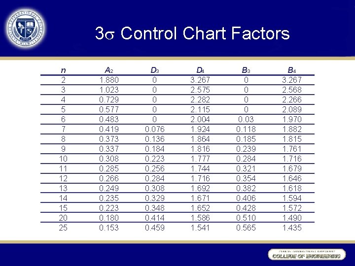
3 Control Chart Factors n 2 3 4 5 6 7 8 9 10 11 12 13 14 15 20 25 A 2 1. 880 1. 023 0. 729 0. 577 0. 483 0. 419 0. 373 0. 337 0. 308 0. 285 0. 266 0. 249 0. 235 0. 223 0. 180 0. 153 D 3 0 0 0. 076 0. 136 0. 184 0. 223 0. 256 0. 284 0. 308 0. 329 0. 348 0. 414 0. 459 D 4 3. 267 2. 575 2. 282 2. 115 2. 004 1. 924 1. 864 1. 816 1. 777 1. 744 1. 716 1. 692 1. 671 1. 652 1. 586 1. 541 B 3 0 0 0. 03 0. 118 0. 185 0. 239 0. 284 0. 321 0. 354 0. 382 0. 406 0. 428 0. 510 0. 565 B 4 3. 267 2. 568 2. 266 2. 089 1. 970 1. 882 1. 815 1. 761 1. 716 1. 679 1. 646 1. 618 1. 594 1. 572 1. 490 1. 435

Example R-Chart 0. 30 Range 0. 25 0. 20 0. 15 0. 10 0. 05 0. 00 1 2 3 4 5 6 Sample 7 8 9 10

Other Variable Charts • MR (Moving Range) Chart – Average of a series of moving ranges – Use difference between successive pairs of numbers in a series • IM (Individual Measurement) Chart

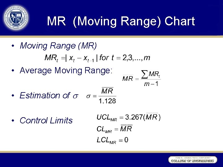
MR (Moving Range) Chart • Moving Range (MR) • Average Moving Range: • Estimation of • Control Limits

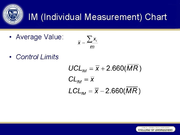
IM (Individual Measurement) Chart • Average Value: • Control Limits

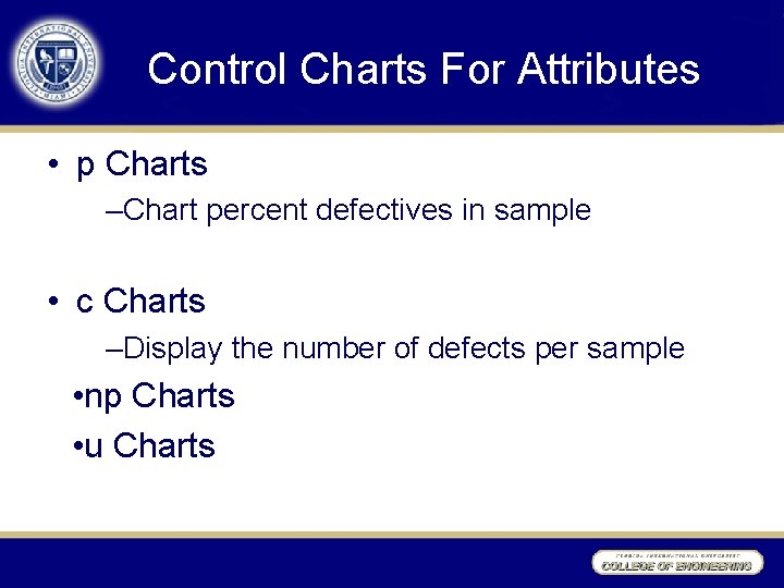
Control Charts For Attributes • p Charts –Chart percent defectives in sample • c Charts –Display the number of defects per sample • np Charts • u Charts

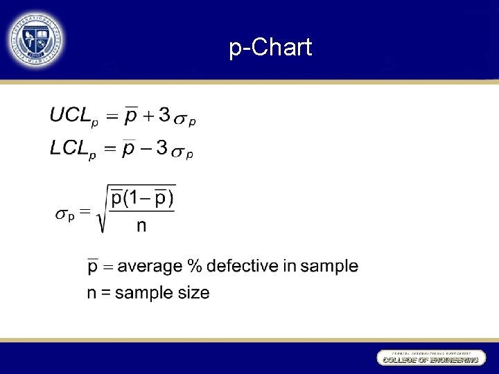
p-Chart

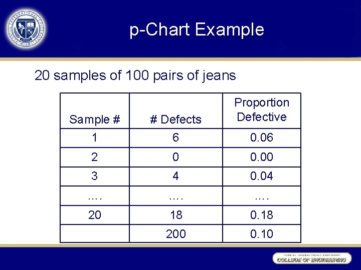
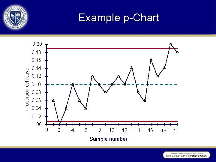
p-Chart Example 20 samples of 100 pairs of jeans Proportion Defective Sample # 1 # Defects 6 2 0 0. 00 3 4 0. 04 …. …. 20 18 0. 18 200 0. 10 0. 06

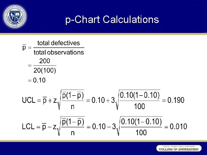
p-Chart Calculations

Example p-Chart 0. 20 0. 18 Proportion defective 0. 16 0. 14 0. 12 0. 10 0. 08 0. 06 0. 04 0. 02 00 0 2 4 6 8 10 12 Sample number 14 16 18 20

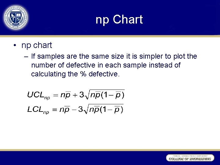
np Chart • np chart – If samples are the same size it is simpler to plot the number of defective in each sample instead of calculating the % defective.

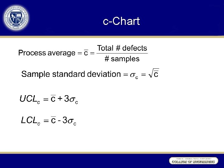
c-Chart

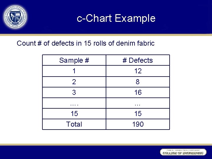
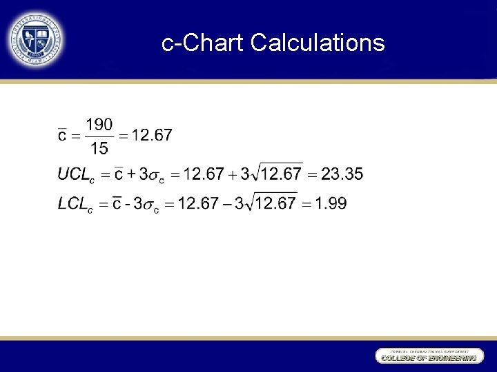
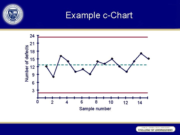
c-Chart Example Count # of defects in 15 rolls of denim fabric Sample # 1 # Defects 12 2 3 8 16 …. 15 Total … 15 190

c-Chart Calculations

Example c-Chart Number of defects 24 21 18 15 12 9 6 3 0 2 4 6 8 10 Sample number 12 14

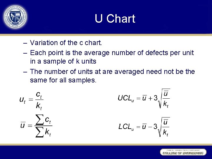
U Chart – Variation of the c chart. – Each point is the average number of defects per unit in a sample of k units – The number of units at are averaged need not be the same for all samples.

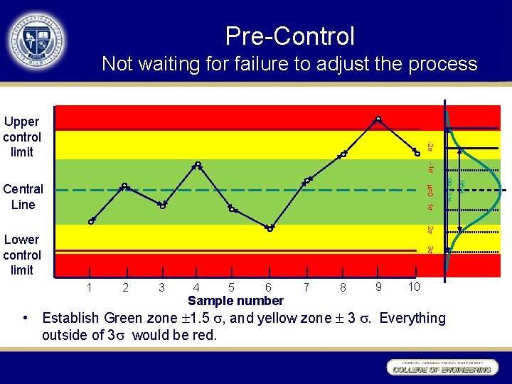
Pre-Control Not waiting for failure to adjust the process -3 Upper control limit -2 -1 2 3 Lower control limit 1 2 3 4 5 6 Sample number 7 8 9 10 • Establish Green zone 1. 5 , and yellow zone 3 . Everything outside of 3 would be red. 95% 99. 73% =0 1 Central Line

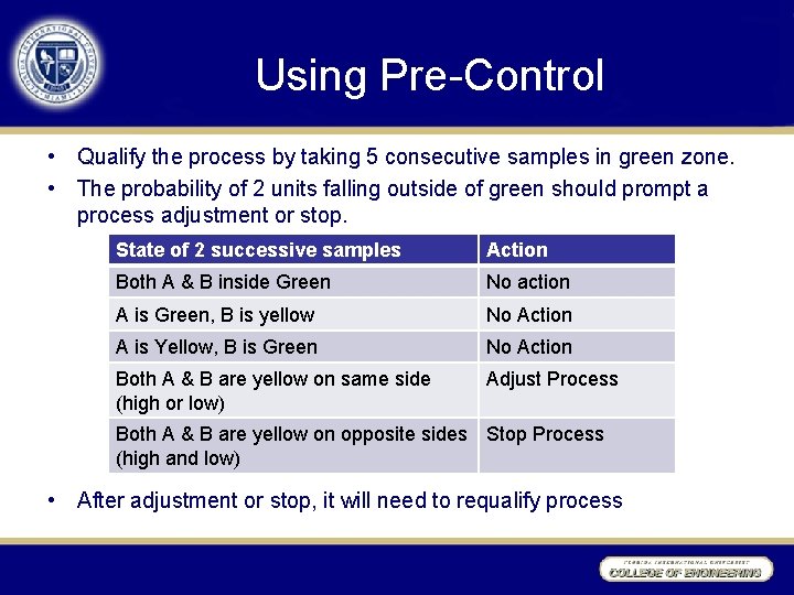
Using Pre-Control • Qualify the process by taking 5 consecutive samples in green zone. • The probability of 2 units falling outside of green should prompt a process adjustment or stop. State of 2 successive samples Action Both A & B inside Green No action A is Green, B is yellow No Action A is Yellow, B is Green No Action Both A & B are yellow on same side (high or low) Adjust Process Both A & B are yellow on opposite sides Stop Process (high and low) • After adjustment or stop, it will need to requalify process