Chapter 15 Capital Structure Decisions Essentials of Managerial

Chapter 15 Capital Structure Decisions Essentials of Managerial Finance by S. Besley & E. Brigham Slide 1 of 24

The Target Capital Structure • Risk—greater risk means greater costs to raise funds • Financial flexibility—a stronger financial position—that is, stronger balance sheet—generally implies the firm is better able to raise funds in the capital markets, especially in slumping economies • Managerial attitude (conservatism or aggressiveness) —some financial managers are more conservative than others when it comes to using debt, thus they are inclined to use less debt, all else equal. Essentials of Managerial Finance by S. Besley & E. Brigham Slide 2 of 24

The Business Risk and Financial Risk • Business Risk—Uncertainty inherent in projections of future returns (ROE or ROA) if the firm uses no debt. • Financial Risk—Additional risk associated with using debt or preferred stock. • Beware: The use of debt intensifies the firm’s business risk borne by the common stockholders. Essentials of Managerial Finance by S. Besley & E. Brigham Slide 3 of 24

Optimal Capital Structure • A firm’s optimal capital structure is a particular mix of debt and equity that maximizes the stock price. • At any point in time, management has a specific target capital structure in mind, presumably the optimal one, although this target may change over time. Essentials of Managerial Finance by S. Besley & E. Brigham Slide 4 of 24

Optimal Capital Structure (cont’d) • We cannot precisely find the best mix of debt and equity in practice • Treat the optimal capital structure as a range – 40% to 50% debt – rather than an exact point, 45%. • Optimal capital structure is unique for each firm depending on its own situation. Essentials of Managerial Finance by S. Besley & E. Brigham Slide 5 of 24

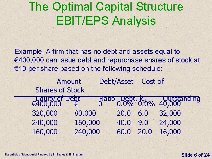
The Optimal Capital Structure EBIT/EPS Analysis Example: A firm that has no debt and assets equal to € 400, 000 can issue debt and repurchase shares of stock at € 10 per share based on the following schedule: Amount Debt/Asset Cost Shares of Stock Equity of Debt Ratio Debt, kd € 400, 000 € 0 0. 0% 320, 000 80, 000 20. 0 6. 0 240, 000 160, 000 40. 0 9. 0 160, 000 240, 000 60. 0 20. 0 Essentials of Managerial Finance by S. Besley & E. Brigham of Outstanding 40, 000 32, 000 24, 000 16, 000 Slide 6 of 24

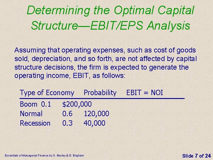
Determining the Optimal Capital Structure—EBIT/EPS Analysis Assuming that operating expenses, such as cost of goods sold, depreciation, and so forth, are not affected by capital structure decisions, the firm is expected to generate the operating income, EBIT, as follows: Type of Economy Boom 0. 1 Normal Recession Probability EBIT = NOI $200, 000 0. 6 120, 000 0. 3 40, 000 Essentials of Managerial Finance by S. Besley & E. Brigham Slide 7 of 24

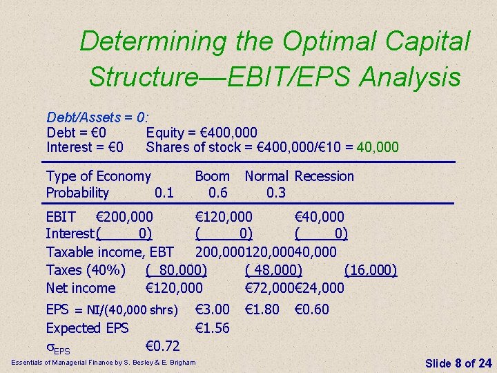
Determining the Optimal Capital Structure—EBIT/EPS Analysis Debt/Assets = 0: Debt = € 0 Equity = € 400, 000 Interest = € 0 Shares of stock = € 400, 000/€ 10 = 40, 000 Type of Economy Probability 0. 1 Boom 0. 6 Normal Recession 0. 3 EBIT € 200, 000 € 120, 000 € 40, 000 Interest (_____0) ( 0) Taxable income, EBT 200, 000120, 00040, 000 Taxes (40%) ( 80, 000) ( 48, 000) (16, 000) Net income € 120, 000 € 72, 000€ 24, 000 EPS = NI/(40, 000 shrs) Expected EPS s. EPS € 0. 72 € 3. 00 € 1. 56 Essentials of Managerial Finance by S. Besley & E. Brigham € 1. 80 € 0. 60 Slide 8 of 24

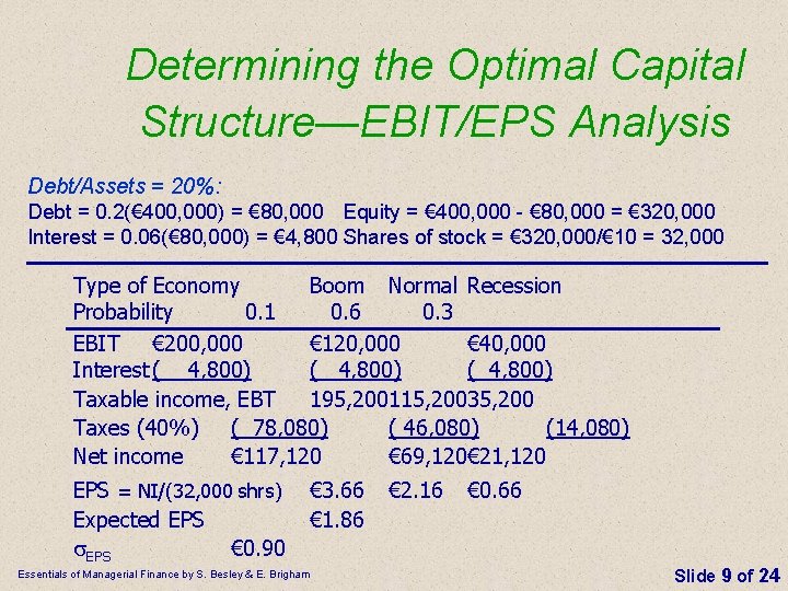
Determining the Optimal Capital Structure—EBIT/EPS Analysis Debt/Assets = 20%: Debt = 0. 2(€ 400, 000) = € 80, 000 Equity = € 400, 000 - € 80, 000 = € 320, 000 Interest = 0. 06(€ 80, 000) = € 4, 800 Shares of stock = € 320, 000/€ 10 = 32, 000 Type of Economy Boom Normal Recession Probability 0. 1 0. 6 0. 3 EBIT € 200, 000 € 120, 000 € 40, 000 Interest ( 4, 800) Taxable income, EBT 195, 200115, 20035, 200 Taxes (40%) ( 78, 080) ( 46, 080) (14, 080) Net income € 117, 120 € 69, 120€ 21, 120 EPS = NI/(32, 000 shrs) Expected EPS s. EPS € 0. 90 € 3. 66 € 1. 86 Essentials of Managerial Finance by S. Besley & E. Brigham € 2. 16 € 0. 66 Slide 9 of 24

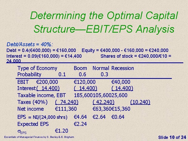
Determining the Optimal Capital Structure—EBIT/EPS Analysis Debt/Assets = 40%: Debt = 0. 4(€ 400, 000) = € 160, 000 Equity = € 400, 000 - € 160, 000 = € 240, 000 Interest = 0. 09(€ 160, 000) = € 14, 400 Shares of stock = € 240, 000/€ 10 = 24, 000 Type of Economy Boom Normal Recession Probability 0. 1 0. 6 0. 3 EBIT € 200, 000 € 120, 000 € 40, 000 Interest ( 14, 400) Taxable income, EBT 185, 600105, 60025, 600 Taxes (40%) ( 74, 240) ( 42, 240) (10, 240) Net income € 111, 360 € 63, 360€ 15, 360 EPS = NI/(24, 000 shrs) Expected EPS s. EPS € 1. 20 € 4. 64 € 2. 24 Essentials of Managerial Finance by S. Besley & E. Brigham € 2. 64 € 0. 64 Slide 10 of 24

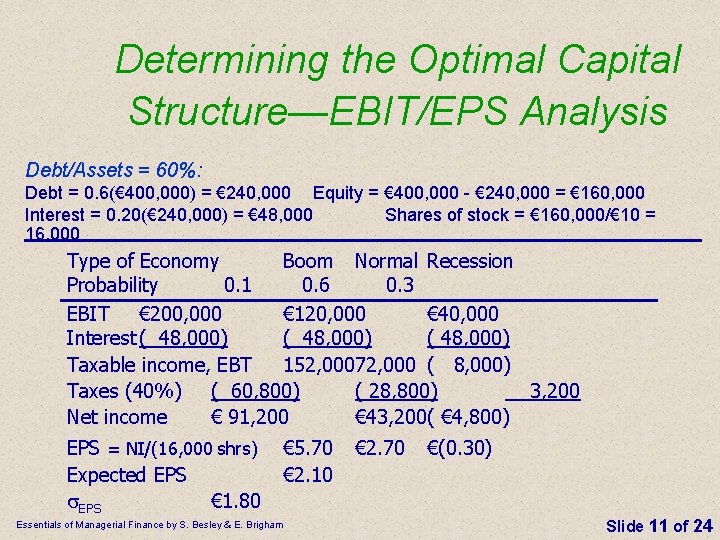
Determining the Optimal Capital Structure—EBIT/EPS Analysis Debt/Assets = 60%: Debt = 0. 6(€ 400, 000) = € 240, 000 Equity = € 400, 000 - € 240, 000 = € 160, 000 Interest = 0. 20(€ 240, 000) = € 48, 000 Shares of stock = € 160, 000/€ 10 = 16, 000 Type of Economy Boom Normal Recession Probability 0. 1 0. 6 0. 3 EBIT € 200, 000 € 120, 000 € 40, 000 Interest ( 48, 000) Taxable income, EBT 152, 00072, 000 ( 8, 000) Taxes (40%) ( 60, 800) ( 28, 800) 3, 200 Net income € 91, 200 € 43, 200( € 4, 800) EPS = NI/(16, 000 shrs) Expected EPS s. EPS € 1. 80 € 5. 70 € 2. 10 Essentials of Managerial Finance by S. Besley & E. Brigham € 2. 70 €(0. 30) Slide 11 of 24

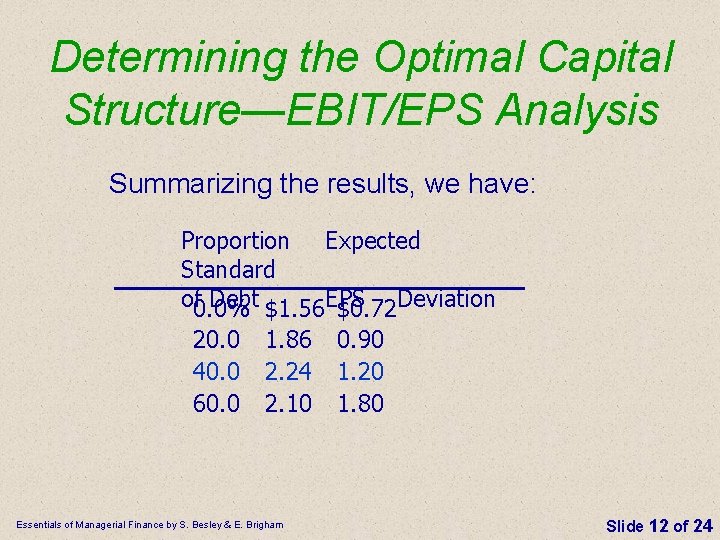
Determining the Optimal Capital Structure—EBIT/EPS Analysis Summarizing the results, we have: Proportion Expected Standard of 0. 0% Debt $1. 56 EPS $0. 72 Deviation 20. 0 40. 0 60. 0 1. 86 2. 24 2. 10 Essentials of Managerial Finance by S. Besley & E. Brigham 0. 90 1. 20 1. 80 Slide 12 of 24

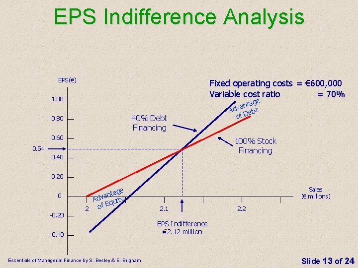
EPS Indifference Analysis EPS(€) Fixed operating costs = € 600, 000 Variable cost ratio = 70% 1. 00 40% Debt Financing 0. 80 0. 60 tage n a v Ad ebt D f o 100% Stock Financing 0. 54 0. 40 0. 20 0 -0. 20 2 tage n a v Ad quity of E -0. 40 Essentials of Managerial Finance by S. Besley & E. Brigham Sales (€ millions) 2. 1 2. 2 EPS Indifference € 2. 12 million Slide 13 of 24

Capital Structure — Stock Price Essentials of Managerial Finance by S. Besley & E. Brigham Slide 14 of 24

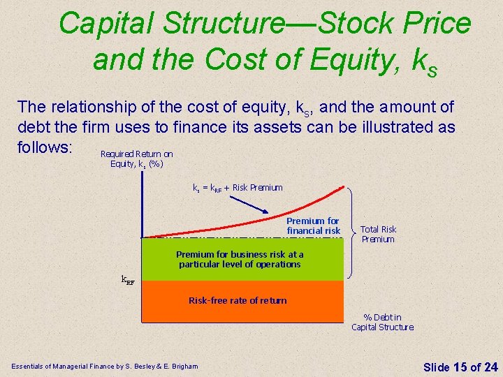
Capital Structure—Stock Price and the Cost of Equity, ks The relationship of the cost of equity, ks, and the amount of debt the firm uses to finance its assets can be illustrated as follows: Required Return on Equity, ks (%) ks = k. RF + Risk Premium for financial risk Total Risk Premium for business risk at a particular level of operations k. RF Risk-free rate of return % Debt in Capital Structure Essentials of Managerial Finance by S. Besley & E. Brigham Slide 15 of 24

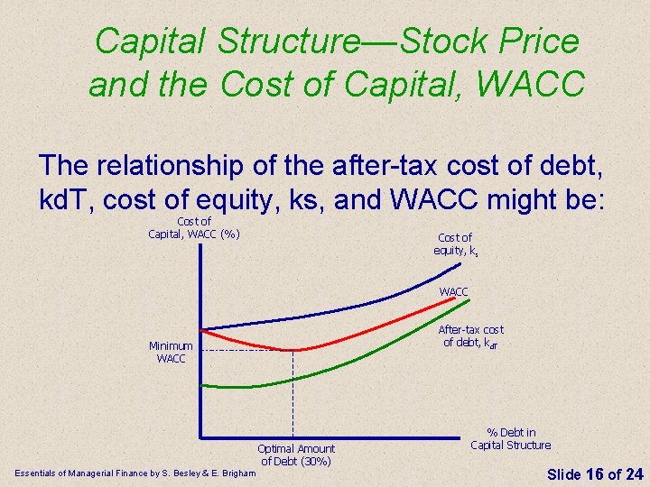
Capital Structure—Stock Price and the Cost of Capital, WACC The relationship of the after-tax cost of debt, kd. T, cost of equity, ks, and WACC might be: Cost of Capital, WACC (%) Cost of equity, ks WACC After-tax cost of debt, kd. T Minimum WACC Optimal Amount of Debt (30%) Essentials of Managerial Finance by S. Besley & E. Brigham % Debt in Capital Structure Slide 16 of 24

Capital Structure - WACC • If the firm uses only equity to finance its assets (that is, zero debt is used) then WACC = ks • As the firm begins to use some debt for financing, WACC declines, primarily because the tax benefit offered by the debt more than offsets the increased cost of equity • At some point the tax benefit associated with debt is more than offset by increases in the before-tax cost of debt and the cost of equity that result from increases in the risk associated with the additional debt and, at this point, WACC begins to increase • The point where WACC is the lowest is the optimal capital structure—this is the point where the value of the firm is maximized Essentials of Managerial Finance by S. Besley & E. Brigham Slide 17 of 24

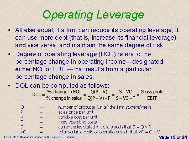
Operating Leverage • All else equal, if a firm can reduce its operating leverage, it can use more debt (that is, increase its financial leverage), and vice versa, and maintain the same degree of risk. • Degree of operating leverage (DOL) refers to the percentage change in operating income—designated either NOI or EBIT—that results from a particular percentage change in sales. • DOL can be computed as follows: number of products (units) the firm currently sells sales price per unit variable cost per unit fixed operating costs current sales stated in dollars such that S = Q P total variable costs of operations such that VC = Q V Essentials of Managerial Finance by S. Besley & E. Brigham Slide 18 of 24 Q P V F S VC = = =

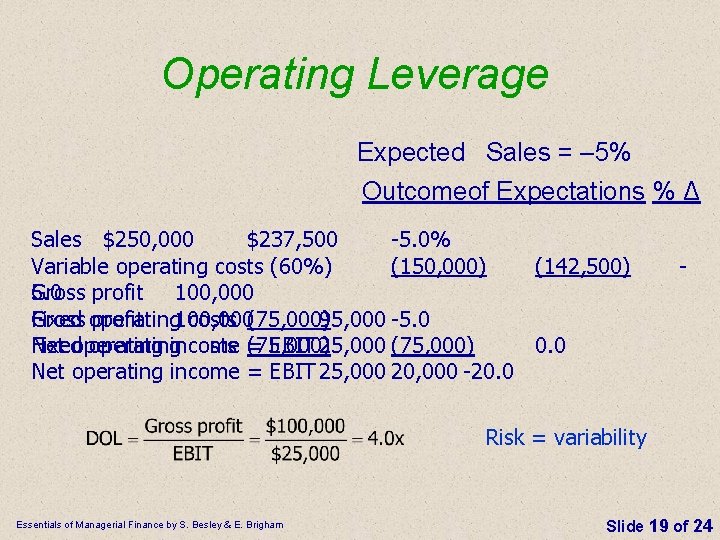
Operating Leverage Expected Sales = – 5% Outcomeof Expectations % Δ Sales $250, 000 $237, 500 -5. 0% Variable operating costs (60%) (150, 000) (142, 500) 5. 0 profit 100, 000 Gross operating Fixed profit 100, 000 costs (75, 000) 95, 000 -5. 0 Fixedoperating Net operatingincome costs = (75, 000) EBIT 25, 000 (75, 000) 0. 0 Net operating income = EBIT 25, 000 20, 000 -20. 0 - Risk = variability Essentials of Managerial Finance by S. Besley & E. Brigham Slide 19 of 24

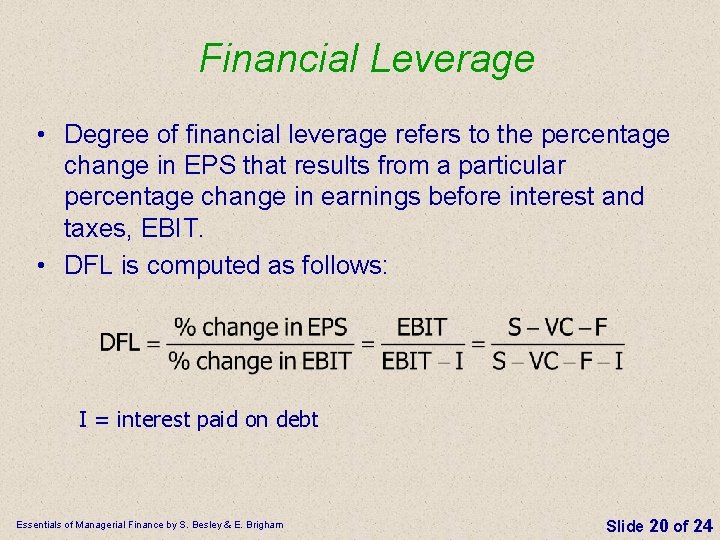
Financial Leverage • Degree of financial leverage refers to the percentage change in EPS that results from a particular percentage change in earnings before interest and taxes, EBIT. • DFL is computed as follows: I = interest paid on debt Essentials of Managerial Finance by S. Besley & E. Brigham Slide 20 of 24

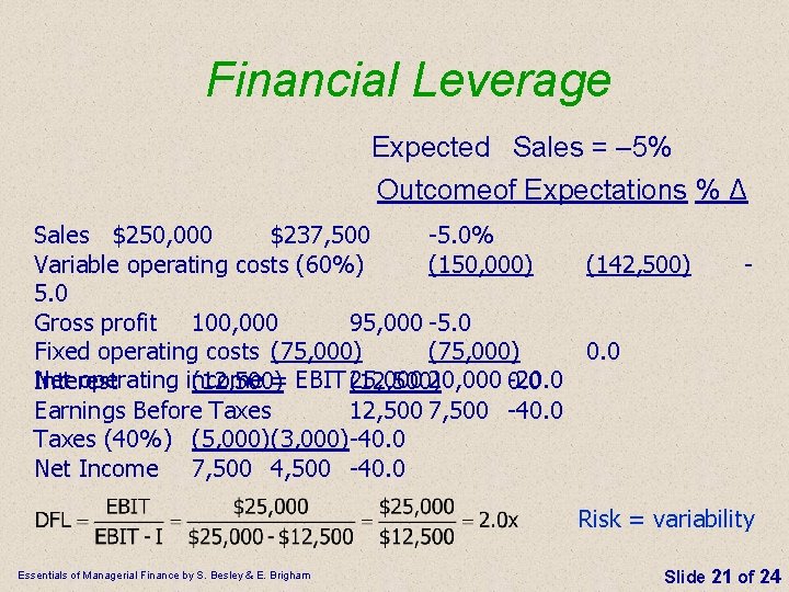
Financial Leverage Expected Sales = – 5% Outcomeof Expectations % Δ Sales $250, 000 $237, 500 -5. 0% Variable operating costs (60%) (150, 000) (142, 500) 5. 0 Gross profit 100, 000 95, 000 -5. 0 Fixed operating costs (75, 000) 0. 0 Net operating income = EBIT (12, 500) 25, 000 20, 000 0. 0 -20. 0 Interest (12, 500) Earnings Before Taxes 12, 500 7, 500 -40. 0 Taxes (40%) (5, 000)(3, 000)-40. 0 (5, 000)(3, 000) Net Income 7, 500 4, 500 -40. 0 - Risk = variability Essentials of Managerial Finance by S. Besley & E. Brigham Slide 21 of 24

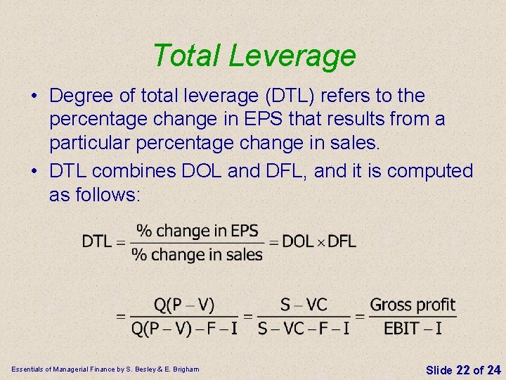
Total Leverage • Degree of total leverage (DTL) refers to the percentage change in EPS that results from a particular percentage change in sales. • DTL combines DOL and DFL, and it is computed as follows: Essentials of Managerial Finance by S. Besley & E. Brigham Slide 22 of 24

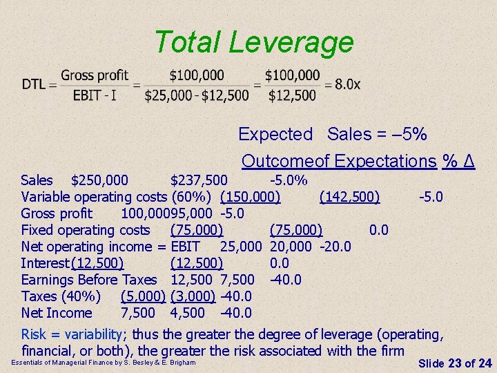
Total Leverage Expected Sales = – 5% Outcomeof Expectations % Δ Sales $250, 000 $237, 500 -5. 0% Variable operating costs (60%) (150, 000) (142, 500) Gross profit 100, 00095, 000 -5. 0 Fixed operating costs (75, 000) 0. 0 Net operating income = EBIT 25, 000 20, 000 -20. 0 Interest (12, 500) 0. 0 Earnings Before Taxes 12, 500 7, 500 -40. 0 Taxes (40%) (5, 000) (3, 000) -40. 0 Net Income 7, 500 4, 500 -40. 0 -5. 0 Risk = variability; thus the greater the degree of leverage (operating, financial, or both), the greater the risk associated with the firm Essentials of Managerial Finance by S. Besley & E. Brigham Slide 23 of 24

Why Does Leveraging Increase Return? • More cash flows are available for investors when the firm borrows. – Total dollars paid to investors: • No debt: NI = $24, 000 • With debt: NI + Interest = $18, 000 + $10, 000 = $28, 000 – Taxes paid: • No debt: $16, 000; With debt: $12, 000 • Equity $ proportionally lower than NI Essentials of Managerial Finance by S. Besley & E. Brigham Slide 24 of 24

Why Does Leveraging Increase Return? (cont’d) • Now consider the fact that EBIT is not known with certainty. Five possible states may arise. What is the impact of uncertainty on stockholder profitability and risk whether or not the firm borrows? Essentials of Managerial Finance by S. Besley & E. Brigham Slide 25 of 24

Liquidity and Capital Structure n A firm might not operate at the optimal capital structure because: n n It might be difficult, if not impossible, to determine the optimal capital structure. Managers might be reluctant to take on the amount of debt necessary to achieve the optimal capital structure —that is, a conservative attitude toward debt might exist. The firm provides important, needed services, and operating at the optimal mix of capital might endanger the firm’s ability to survive. Financial liquidity is important to such firms. Essentials of Managerial Finance by S. Besley & E. Brigham Slide 26 of 24

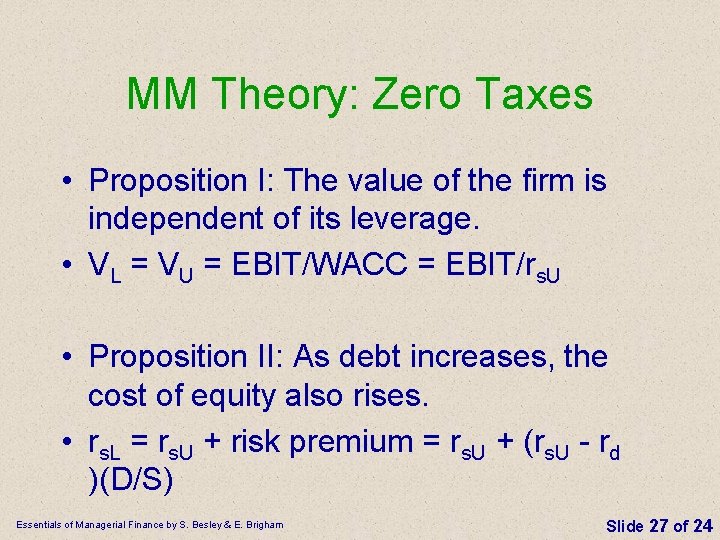
MM Theory: Zero Taxes • Proposition I: The value of the firm is independent of its leverage. • VL = VU = EBIT/WACC = EBIT/rs. U • Proposition II: As debt increases, the cost of equity also rises. • rs. L = rs. U + risk premium = rs. U + (rs. U - rd )(D/S) Essentials of Managerial Finance by S. Besley & E. Brigham Slide 27 of 24

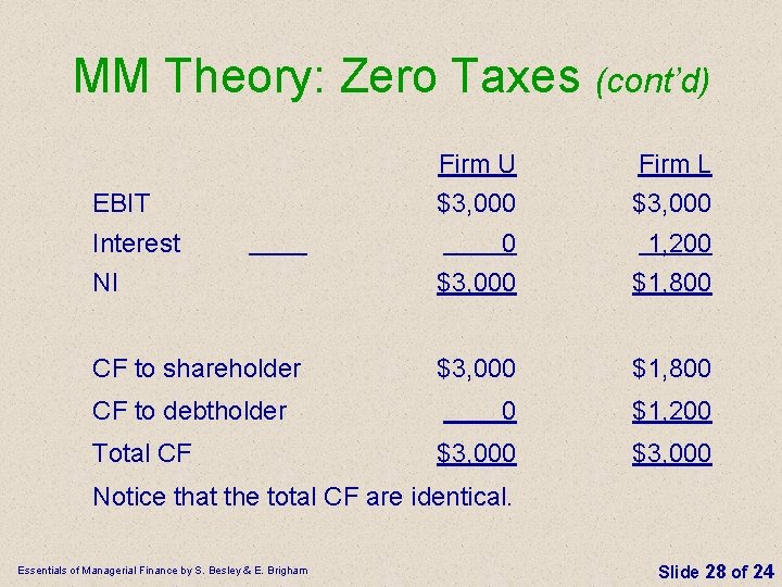
MM Theory: Zero Taxes (cont’d) Firm U Firm L $3, 000 0 1, 200 NI $3, 000 $1, 800 CF to shareholder $3, 000 $1, 800 0 $1, 200 $3, 000 EBIT Interest CF to debtholder Total CF Notice that the total CF are identical. Essentials of Managerial Finance by S. Besley & E. Brigham Slide 28 of 24

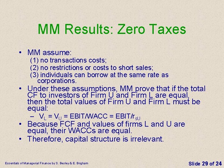
MM Results: Zero Taxes • MM assume: (1) no transactions costs; (2) no restrictions or costs to short sales; (3) individuals can borrow at the same rate as corporations. • Under these assumptions, MM prove that if the total CF to investors of Firm U and Firm L are equal, then the total values of Firm U and Firm L must be equal: – VL = VU = EBIT/WACC = EBIT/rs. U • Because FCF and values of firms L and U are equal, their WACCs are equal. • Therefore, capital structure is irrelevant. Essentials of Managerial Finance by S. Besley & E. Brigham Slide 29 of 24

MM’s Arbitrage Proof • Arbitrage means the simultaneous buying and selling of essentially identical assets that sell at different prices. • The buying increases the price of the undervalued asset, and the selling decreases the price of the overvalued asset. • Arbitrage operations will continue until prices have adjusted to the point where profit is zero, at which point the market is in equilibrium. With no transaction costs, equilibrium requires that the prices of the two assets be equal. Essentials of Managerial Finance by S. Besley & E. Brigham Slide 30 of 24

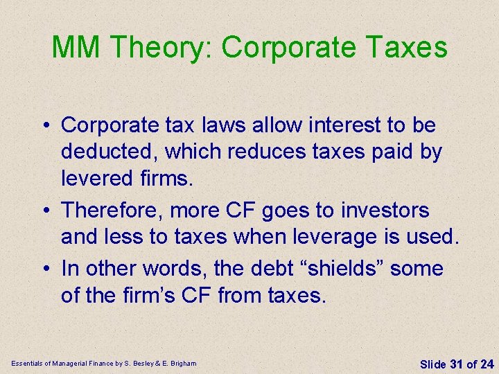
MM Theory: Corporate Taxes • Corporate tax laws allow interest to be deducted, which reduces taxes paid by levered firms. • Therefore, more CF goes to investors and less to taxes when leverage is used. • In other words, the debt “shields” some of the firm’s CF from taxes. Essentials of Managerial Finance by S. Besley & E. Brigham Slide 31 of 24

MM Result: Corporate Taxes • MM show that the total CF to Firm L’s investors is equal to the total CF to Firm U’s investor, plus an additional amount due to interest deductibility: CFL = CFU + (rd. D)T. • MM then show that: VL = VU + TD. • If T= 40%, then every dollar of debt adds 40 cents of extra value to firm. Essentials of Managerial Finance by S. Besley & E. Brigham Slide 32 of 24

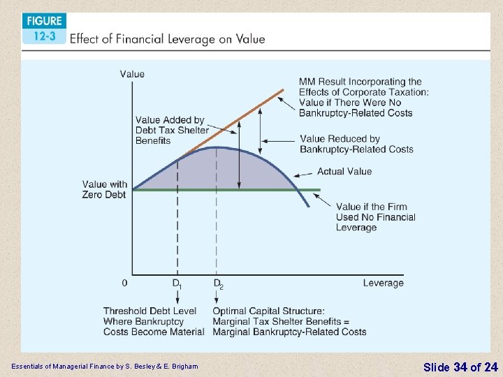
Capital Structure—Trade-Off Theory • The value of a firm increases as it uses more and more debt. • Ignores the costs associated with bankruptcy, which can be considerable • If bankruptcy costs are considered, there is a point where the benefit of the tax deductibility of debt is more than offset by increases in the cost of debt and the cost of equity that result from the risk associated with the firm’s heavy use of debt Essentials of Managerial Finance by S. Besley & E. Brigham Slide 33 of 24

Essentials of Managerial Finance by S. Besley & E. Brigham Slide 34 of 24

Capital Structure—Signaling Theory • Studies have shown that when firms issue new common stock to raise funds the per share value of the stock decreases. – Perhaps this occurs because managers would only issue new common stock if they felt that the firm’s future prospects were unfavorable. – When debt is issued, only the contracted costs need to be paid—that is, fixed interest and the repayment of the debt—and the remaining gains from the favorable projects accrue to the stockholders. – Age of a firm—younger firms generally do not have the same access to financial markets as older, more established firms Essentials of Managerial Finance by S. Besley & E. Brigham Slide 35 of 24