Chapter 15 B External Methods BTrees BTrees To

Chapter 15 B External Methods – B-Trees

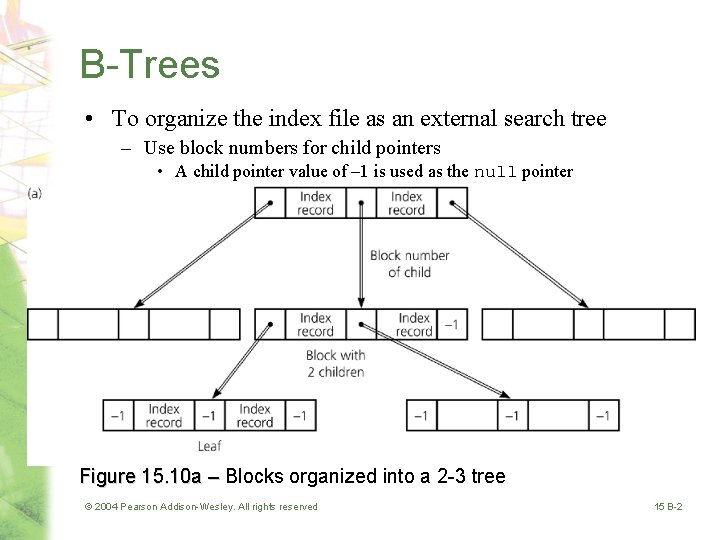
B-Trees • To organize the index file as an external search tree – Use block numbers for child pointers • A child pointer value of – 1 is used as the null pointer Figure 15. 10 a – Blocks organized into a 2 -3 tree © 2004 Pearson Addison-Wesley. All rights reserved 15 B-2

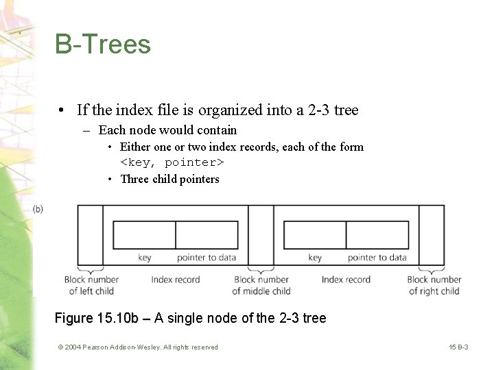
B-Trees • If the index file is organized into a 2 -3 tree – Each node would contain • Either one or two index records, each of the form <key, pointer> • Three child pointers Figure 15. 10 b – A single node of the 2 -3 tree © 2004 Pearson Addison-Wesley. All rights reserved 15 B-3

B-Trees • An external 2 -3 tree is adequate, but an improvement is possible • To improve efficiency – Allow each node to have as many children as possible • In an external environment, the advantage of keeping a search tree short far outweighs the disadvantage of performing extra work at each node • Block size should be the only limiting factor for the number of children © 2004 Pearson Addison-Wesley. All rights reserved 15 B-4

B-Trees • Binary search tree – If a node N has two children, it must contain one key value • 2 -3 tree – If a node N has three children, it must contain two key values • General search tree – If a node N has m children, it must contain m – 1 key values © 2004 Pearson Addison-Wesley. All rights reserved 15 B-5

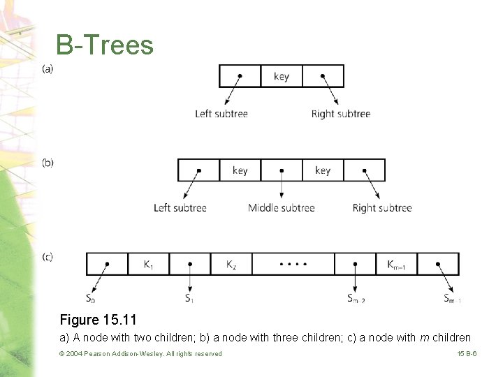
B-Trees Figure 15. 11 a) A node with two children; b) a node with

B-Trees • B-tree of degree m – All leaves are at the same level – Nodes • Each node contains between m – 1 and m/2 records • Each internal node has one more child than it has records • Exception: The root can contain as few as one record and can have as few as two children – Example • A 2 -3 tree is a B-tree of degree 3 – Each node contains between (3 -1) = 2 and 3/2 = 1 records. © 2004 Pearson Addison-Wesley. All rights reserved 15 B-7

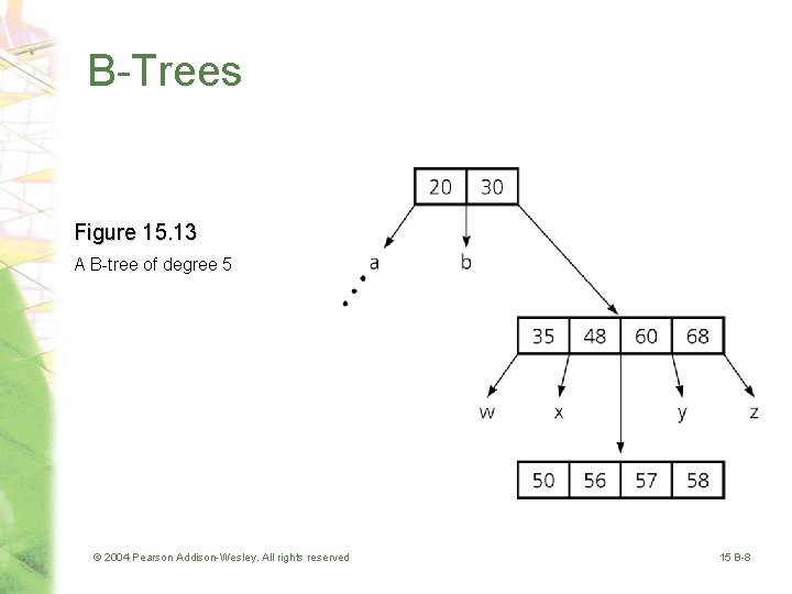
B-Trees Figure 15. 13 A B-tree of degree 5 © 2004 Pearson Addison-Wesley. All

B-Trees • Retrieval – Generalized search tree retrieval • Insertion into a B-tree – Step 1: Insert the data record into the data file – Step 2: Insert a corresponding index record into the index file © 2004 Pearson Addison-Wesley. All rights reserved 15 B-9

B-Trees Figure 15. 14 a and b The steps for inserting 55 © 2004

B-Trees Figure 15. 14 c-e The steps for inserting 55 © 2004 Pearson Addison-Wesley.

B-Trees • Deletion from a B-tree – Step 1: Locate the index record in the index file and delete it from the index file – Step 2: Delete the data record from the data file © 2004 Pearson Addison-Wesley. All rights reserved 15 B-12

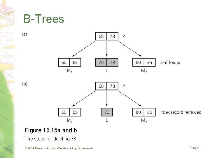
B-Trees Figure 15. 15 a and b The steps for deleting 73 © 2004

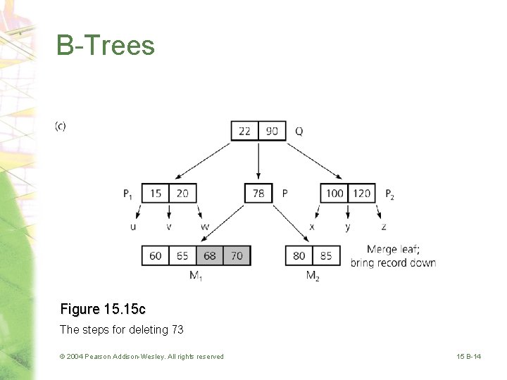
B-Trees Figure 15. 15 c The steps for deleting 73 © 2004 Pearson Addison-Wesley.

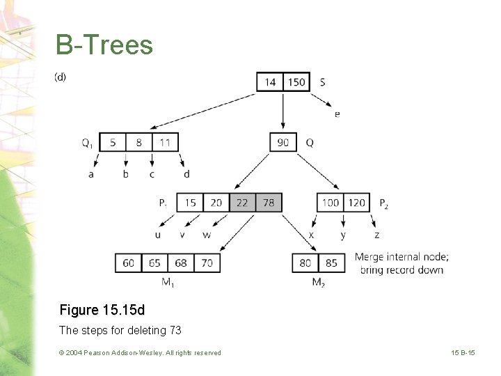
B-Trees Figure 15. 15 d The steps for deleting 73 © 2004 Pearson Addison-Wesley.

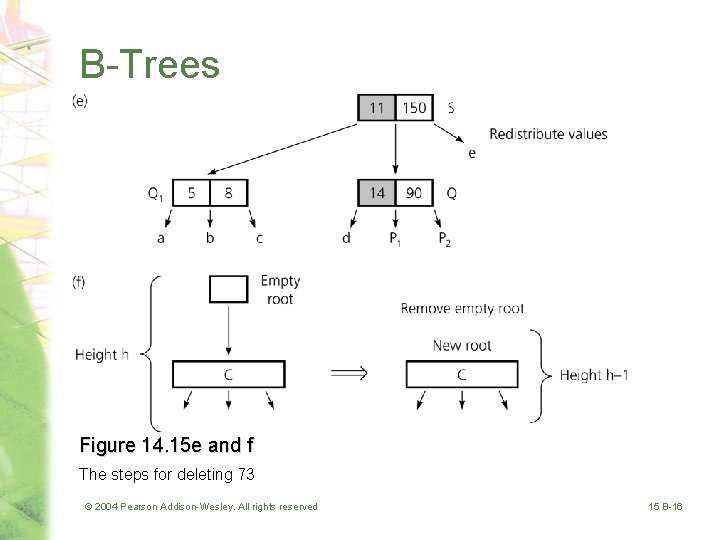
B-Trees Figure 14. 15 e and f The steps for deleting 73 © 2004

Traversals • Accessing only the search key of each record, not the data file – Not efficiently supported by the hashing implementation – Efficiently supported by the B-tree implementation • The search keys can be visited in sorted order by using an inorder traversal of the B-tree • Accessing the entire data record – Not efficiently supported by the B-tree implementation © 2004 Pearson Addison-Wesley. All rights reserved 15 B-17

Multiple Indexing • Advantage – Allows multiple data organizations • Disadvantage – More storage space – Additional overhead for updating each index whenever the data file is modified © 2004 Pearson Addison-Wesley. All rights reserved 15 B-18

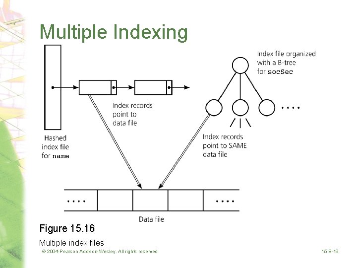
Multiple Indexing Figure 15. 16 Multiple index files © 2004 Pearson Addison-Wesley. All rights

Variations of B-Trees • The fewer nodes are in a B-tree, the better. (Why? ) • Problems of B-tree: – It could be only half full • More nodes required • Space wasted – Inorder traversal “jumps” around nodes • B*-Trees: introduced by Donald Knuth • B+-Trees: introduced by H. Wedekind Chi-Cheng Lin, Winona State University 20

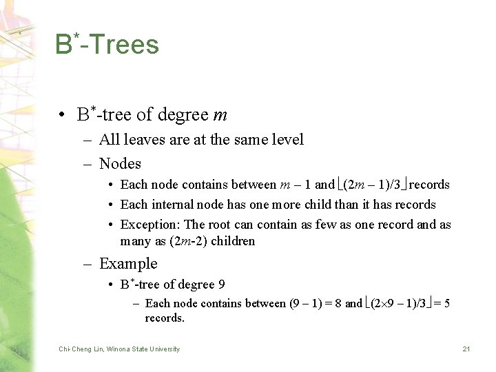
B*-Trees • B*-tree of degree m – All leaves are at the same level – Nodes • Each node contains between m – 1 and (2 m – 1)/3 records • Each internal node has one more child than it has records • Exception: The root can contain as few as one record and as many as (2 m-2) children – Example • B*-tree of degree 9 – Each node contains between (9 – 1) = 8 and (2 9 – 1)/3 = 5 records. Chi-Cheng Lin, Winona State University 21

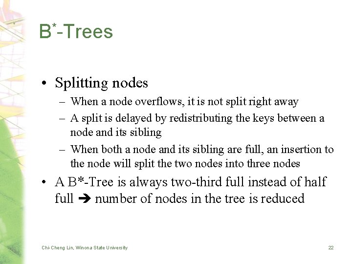
B*-Trees • Splitting nodes – When a node overflows, it is not split right away – A split is delayed by redistributing the keys between a node and its sibling – When both a node and its sibling are full, an insertion to the node will split the two nodes into three nodes • A B*-Tree is always two-third full instead of half full number of nodes in the tree is reduced Chi-Cheng Lin, Winona State University 22

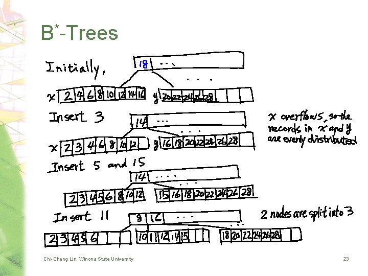
B*-Trees Chi-Cheng Lin, Winona State University 23

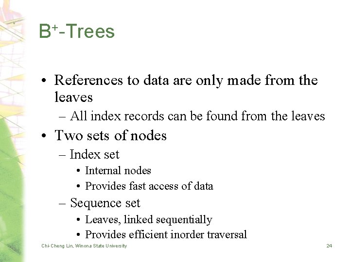
B+-Trees • References to data are only made from the leaves – All index records can be found from the leaves • Two sets of nodes – Index set • Internal nodes • Provides fast access of data – Sequence set • Leaves, linked sequentially • Provides efficient inorder traversal Chi-Cheng Lin, Winona State University 24

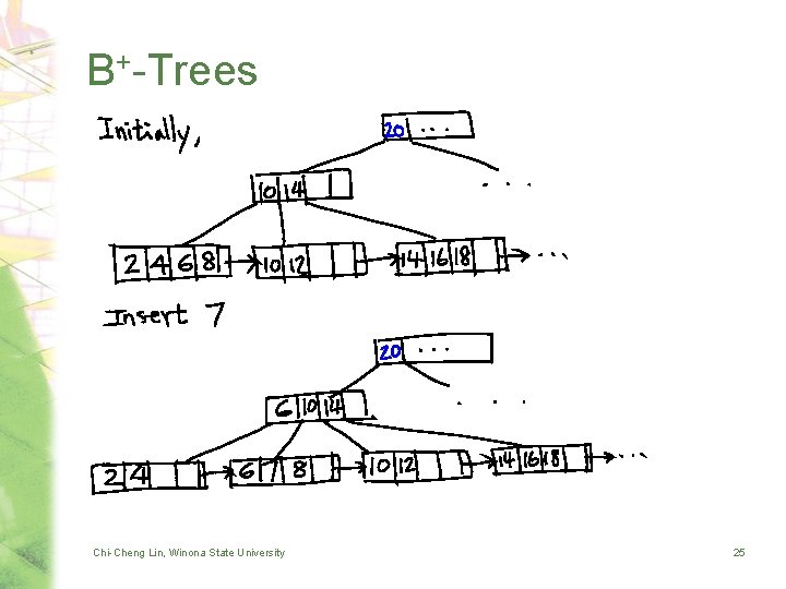
B+-Trees Chi-Cheng Lin, Winona State University 25