Chapter 15 Analysis of Variance 15 1 Introduction

Chapter 15 Analysis of Variance

15. 1 Introduction • Analysis of variance compares two or more populations of interval data. • Specifically, we are interested in determining whether differences exist between the population means. • The procedure works by analyzing the sample variance.

15. 2 One Way Analysis of Variance • The analysis of variance is a procedure that tests to determine whether differences exits between two or more population means. • To do this, the technique analyzes the sample variances

One Way Analysis of Variance • Example 15. 1 – An apple juice manufacturer is planning to develop a new product -a liquid concentrate. – The marketing manager has to decide how to market the new product. – Three strategies are considered • Emphasize convenience of using the product. • Emphasize the quality of the product. • Emphasize the product’s low price.

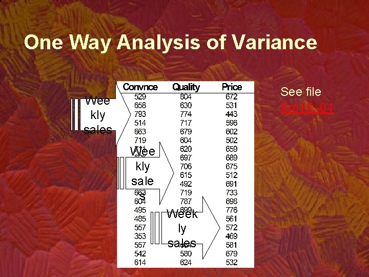
One Way Analysis of Variance • Example 15. 1 - continued – An experiment was conducted as follows: • In three cities an advertisement campaign was launched. • In each city only one of the three characteristics (convenience, quality, and price) was emphasized. • The weekly sales were recorded for twenty weeks following the beginning of the campaigns.

One Way Analysis of Variance See file Xm 15 -01 Wee kly sales Wee kly sale s Week ly sales

One Way Analysis of Variance • Solution – The data are interval – The problem objective is to compare sales in three cities. – We hypothesize that the three population means are equal

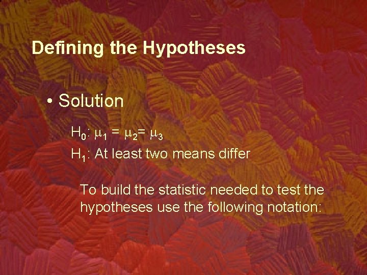
Defining the Hypotheses • Solution H 0: m 1 = m 2= m 3 H 1: At least two means differ To build the statistic needed to test the hypotheses use the following notation:

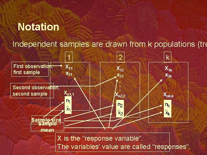
Notation Independent samples are drawn from k populations (tre 1 First observation, first sample X 11 x 21. . . Second observation, Xn 1, 1 second sample 2 k X 12 x 22. . . Xn 2, 2 X 1 k x 2 k. . . Xnk, k Sample size Sample mean X is the “response variable”. The variables’ value are called “responses”.

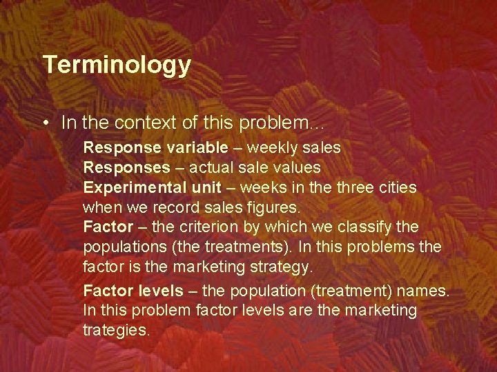
Terminology • In the context of this problem… Response variable – weekly sales Responses – actual sale values Experimental unit – weeks in the three cities when we record sales figures. Factor – the criterion by which we classify the populations (the treatments). In this problems the factor is the marketing strategy. Factor levels – the population (treatment) names. In this problem factor levels are the marketing trategies.

The rationale of the test statistic Two types of variability are employed when testing for the equality of the population means

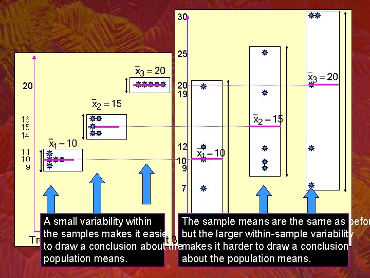
Graphical demonstration: Employing two types of variability

30 25 20 20 19 16 15 14 11 10 9 12 10 9 7 A small variability within The sample means are the same as befor 1 the samples makes it easier but the larger within-sample variability Treatment 1 Treatment 2 3 Treatment 1 Treatment 2 Treatment 3 to draw a conclusion about themakes it harder to draw a conclusion population means. about the population means.

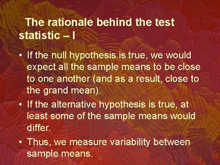
The rationale behind the test statistic – I • If the null hypothesis is true, we would expect all the sample means to be close to one another (and as a result, close to the grand mean). • If the alternative hypothesis is true, at least some of the sample means would differ. • Thus, we measure variability between sample means.

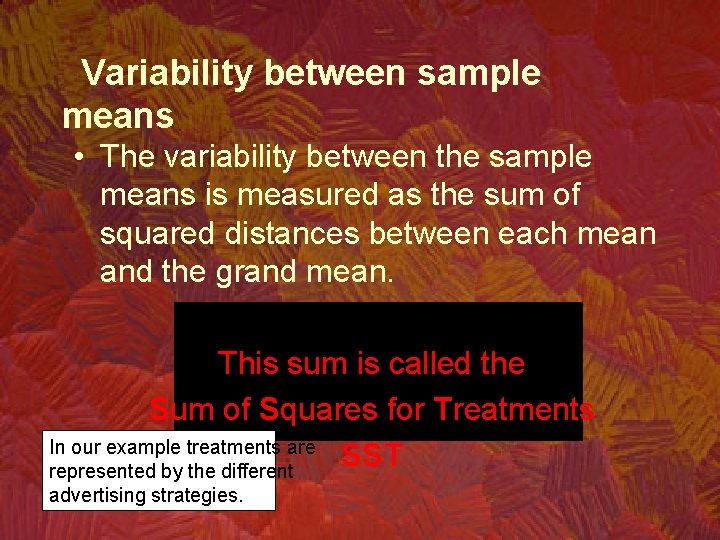
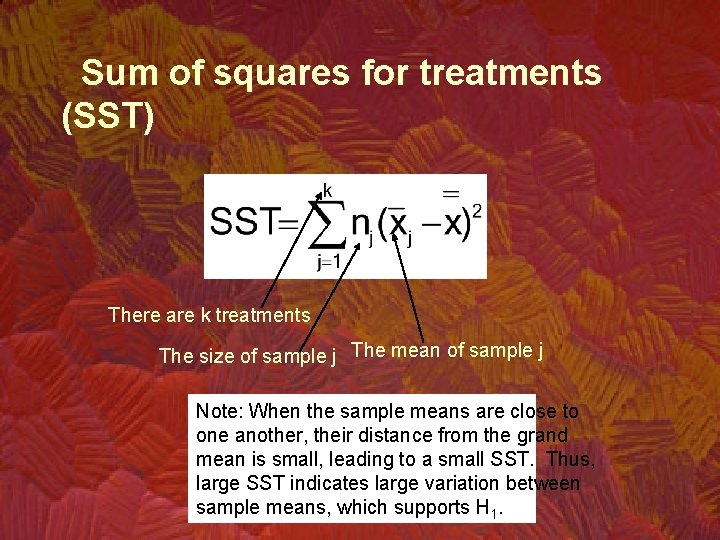
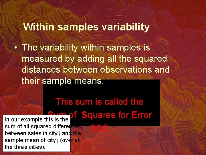
Variability between sample means • The variability between the sample means is measured as the sum of squared distances between each mean and the grand mean. This sum is called the Sum of Squares for Treatments In our example treatments are SST represented by the different advertising strategies.

Sum of squares for treatments (SST) There are k treatments The size of sample j The mean of sample j Note: When the sample means are close to one another, their distance from the grand mean is small, leading to a small SST. Thus, large SST indicates large variation between sample means, which supports H 1.

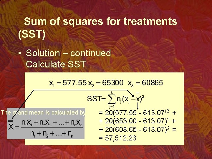
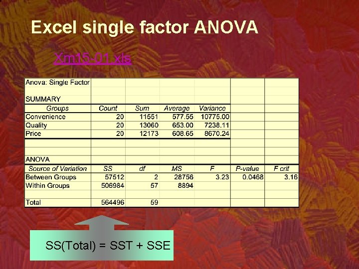
Sum of squares for treatments (SST) • Solution – continued Calculate SST The grand mean is calculated by = 20(577. 55 - 613. 07)2 + + 20(653. 00 - 613. 07)2 + + 20(608. 65 - 613. 07)2 = = 57, 512. 23

Sum of squares for treatments (SST) Is SST = 57, 512. 23 large enough to reject H 0 in favor of H 1? See next.

The rationale behind test statistic – II • Large variability within the samples weakens the “ability” of the sample means to represent their corresponding population means. • Therefore, even though sample means may markedly differ from one another, SST must be judged relative to the “within samples variability”.

Within samples variability • The variability within samples is measured by adding all the squared distances between observations and their sample means. This sum is called the Sum of Squares for Error In our example this is the sum of all squared differences SSE between sales in city j and the sample mean of city j (over all the three cities).

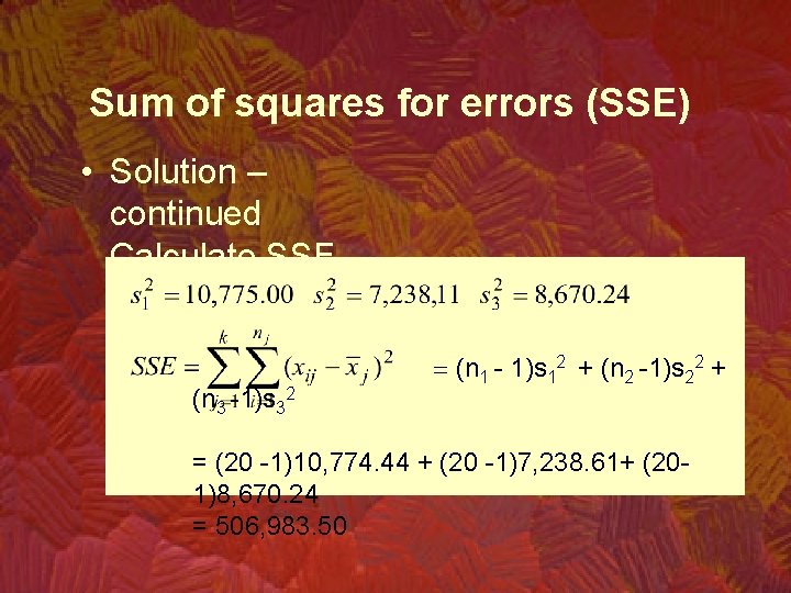
Sum of squares for errors (SSE) • Solution – continued Calculate SSE (n 3 -1)s 32 = (n 1 - 1)s 12 + (n 2 -1)s 22 + = (20 -1)10, 774. 44 + (20 -1)7, 238. 61+ (201)8, 670. 24 = 506, 983. 50

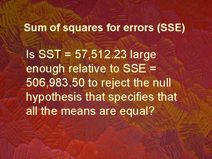
Sum of squares for errors (SSE) Is SST = 57, 512. 23 large enough relative to SSE = 506, 983. 50 to reject the null hypothesis that specifies that all the means are equal?

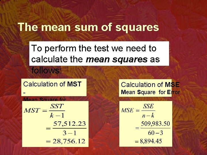
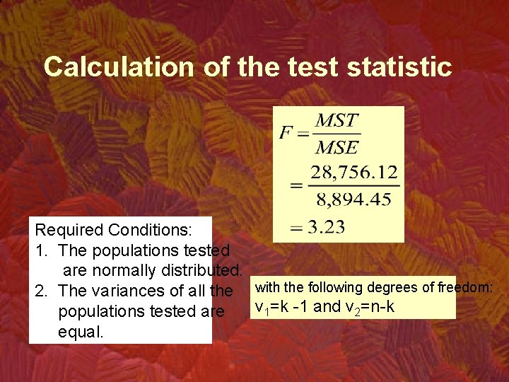
The mean sum of squares To perform the test we need to calculate the mean squares as follows: Calculation of MST Mean Square for Treatments Calculation of MSE Mean Square for Error

Calculation of the test statistic Required Conditions: 1. The populations tested are normally distributed. 2. The variances of all the with the following degrees of freedom: v 1=k -1 and v 2=n-k populations tested are equal.

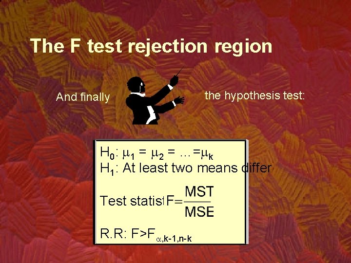
The F test rejection region And finally the hypothesis test: H 0: m 1 = m 2 = …=mk H 1: At least two means differ Test statistic: R. R: F>Fa, k-1, n-k

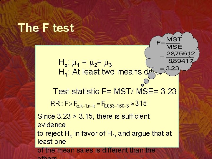
The F test H o: m 1 = m 2= m 3 H 1: At least two means differ Test statistic F= MST/ MSE= 3. 23 Since 3. 23 > 3. 15, there is sufficient evidence to reject Ho in favor of H 1, and argue that at least one of the mean sales is different than the

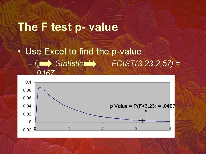
The F test p- value • Use Excel to find the p-value – fx Statistical. 0467 FDIST(3. 23, 2, 57) = p Value = P(F>3. 23) =. 0467

Excel single factor ANOVA Xm 15 -01. xls SS(Total) = SST + SSE

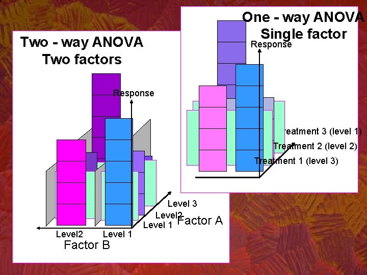
15. 3 Analysis of Variance Experimental Designs • Several elements may distinguish between one experimental design and others. – The number of factors. • Each characteristic investigated is called a factor. • Each factor has several levels.

One - way ANOVA Single factor Two - way ANOVA Two factors Response Treatment 3 (level 1) Treatment 2 (level 2) Treatment 1 (level 3) Level 2 Level 1 Factor B Level 3 Level 2 Level 1 Factor A

Independent samples or blocks • Groups of matched observations are formed into blocks, in order to remove the effects of “unwanted” variability. • By doing so we improve the chances of detecting the variability of interest.

Models of Fixed and Random Effects • Fixed effects – If all possible levels of a factor are included in our analysis we have a fixed effect ANOVA. – The conclusion of a fixed effect ANOVA applies only to the levels studied. • Random effects – If the levels included in our analysis represent a random sample of all the possible levels, we have a random-effect ANOVA. – The conclusion of the random-effect ANOVA applies to all the levels (not only those studied).

Models of Fixed and Random Effects. • In some ANOVA models the test statistic of the fixed effects case may differ from the test statistic of the random effect case. • Fixed and random effects - examples – Fixed effects - The advertisement Example (15. 1): All the levels of the marketing strategies were included – Random effects - To determine if there is a difference in the production rate of 50 machines, four machines are randomly selected and there production recorded.

15. 4 Randomized Blocks (Two-way) Analysis of Variance • The purpose of designing a randomized block experiment is to reduce the withintreatments variation thus increasing the relative amount of between treatment variation. • This helps in detecting differences between the treatment means more easily.

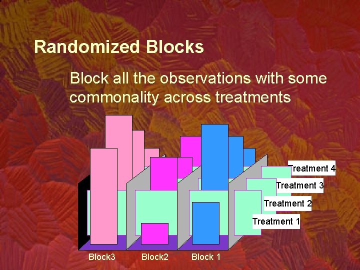
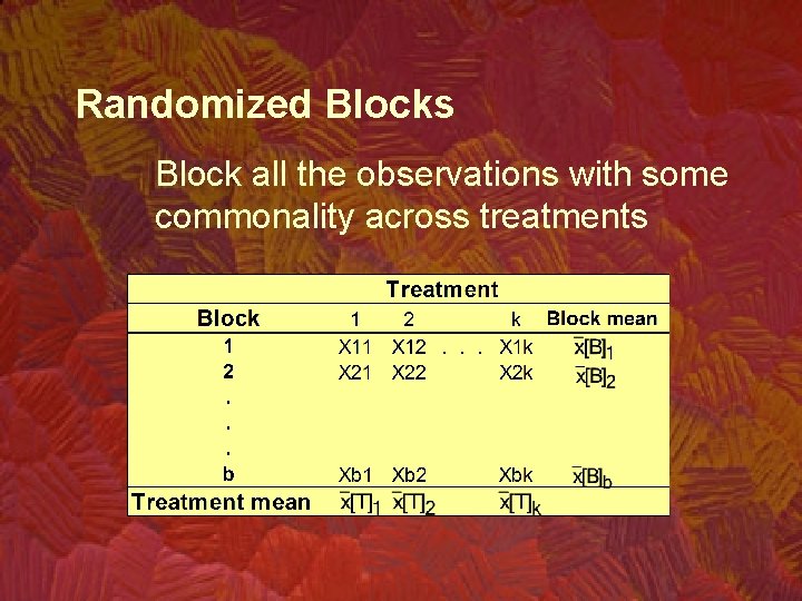
Randomized Blocks Block all the observations with some commonality across treatments Treatment 4 Treatment 3 Treatment 2 Treatment 1 Block 3 Block 2 Block 1

Randomized Blocks Block all the observations with some commonality across treatments

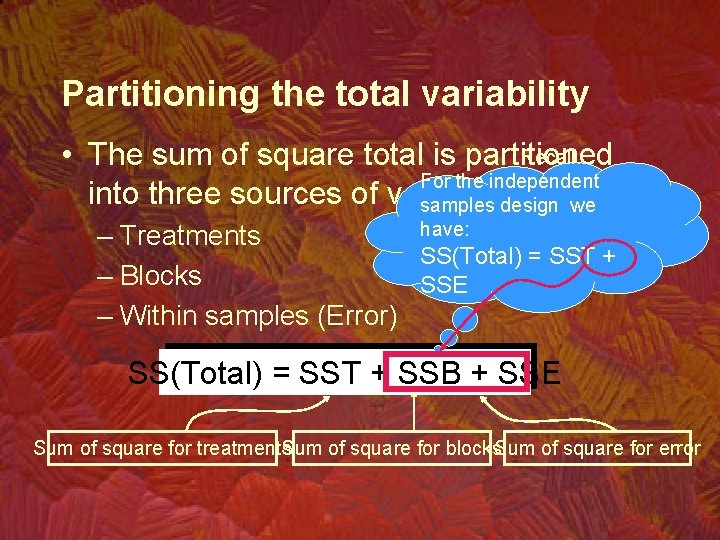
Partitioning the total variability Recall. • The sum of square total is partitioned For the independent into three sources of variation samples design we have: – Treatments SS(Total) = SST + – Blocks SSE – Within samples (Error) SS(Total) = SST + SSB + SSE Sum of square for treatments Sum of square for blocks. Sum of square for error

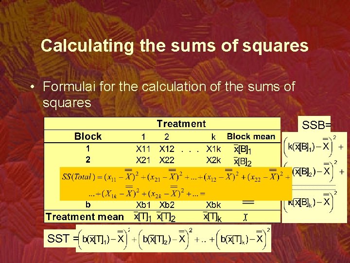
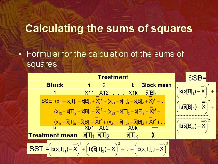
Calculating the sums of squares • Formulai for the calculation of the sums of squares SSB= SST =

Calculating the sums of squares • Formulai for the calculation of the sums of squares SSB= SST =

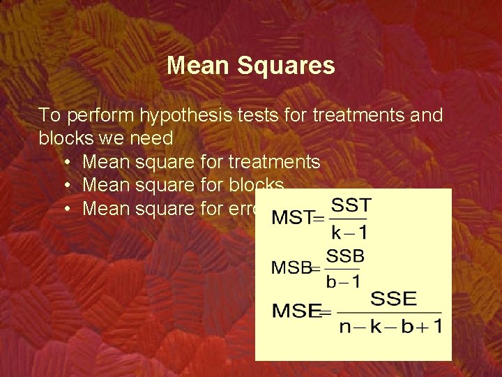
Mean Squares To perform hypothesis tests for treatments and blocks we need • Mean square for treatments • Mean square for blocks • Mean square for error

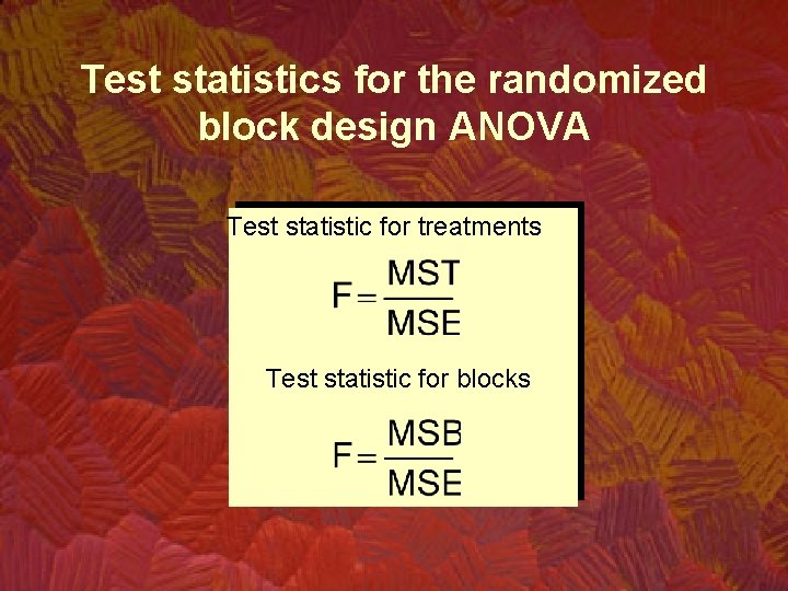
Test statistics for the randomized block design ANOVA Test statistic for treatments Test statistic for blocks

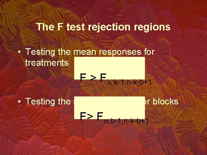
The F test rejection regions • Testing the mean responses for treatments F > Fa, k-1, n-k-b+1 • Testing the mean response for blocks F> Fa, b-1, n-k-b+1

Randomized Blocks ANOVA Example • Example 15. 2 – Are there differences in the effectiveness of cholesterol reduction drugs? – To answer this question the following experiment was organized: • 25 groups of men with high cholesterol were matched by age and weight. Each group consisted of 4 men. • Each person in a group received a different drug. • The cholesterol level reduction in two months was recorded. – Can we infer from the data in Xm 15 -02 that there are differences in mean cholesterol

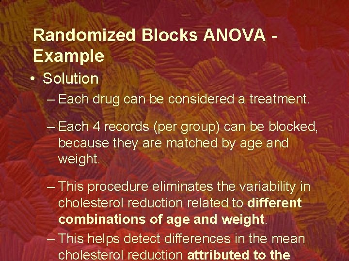
Randomized Blocks ANOVA Example • Solution – Each drug can be considered a treatment. – Each 4 records (per group) can be blocked, because they are matched by age and weight. – This procedure eliminates the variability in cholesterol reduction related to different combinations of age and weight. – This helps detect differences in the mean cholesterol reduction attributed to the

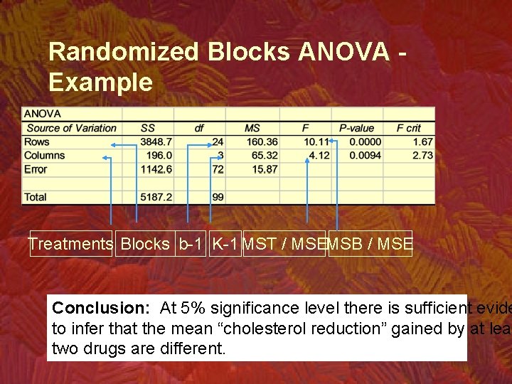
Randomized Blocks ANOVA Example Treatments Blocks b-1 K-1 MST / MSEMSB / MSE Conclusion: At 5% significance level there is sufficient evide to infer that the mean “cholesterol reduction” gained by at leas two drugs are different.