Chapter 14 Query Optimization Chapter 14 Query Optimization

Chapter 14 Query Optimization

Chapter 14: Query Optimization n Introduction n Statistical (Catalog) Information for Cost Estimation n Estimation of Statistics n Cost-based vs. rule-based optimization n Revisiting Selection Algorithms n Transformation of Relational Expressions and Equivalence rules n Dynamic Programming for Choosing Evaluation Plans n Optimizing nested subqueries n Materialized views and view maintenance Database System Concepts 3 rd Edition 14. 2 ©Silberschatz, Korth and Sudarshan

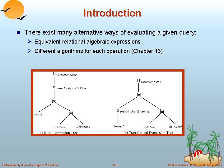
Introduction n There exist many alternative ways of evaluating a given query: Ø Equivalent relational algebraic expressions Ø Different algorithms for each operation (Chapter 13) Database System Concepts 3 rd Edition 14. 3 ©Silberschatz, Korth and Sudarshan

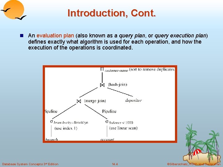
Introduction, Cont. n An evaluation plan (also known as a query plan, or query execution plan) defines exactly what algorithm is used for each operation, and how the execution of the operations is coordinated. Database System Concepts 3 rd Edition 14. 4 ©Silberschatz, Korth and Sudarshan

Introduction, Cont. n Cost difference between different plans can be enormous: Ø Example: performing a r X s followed by a selection r. A = s. B is much slower than performing a join on the same condition. n Optimizer frequently estimates the cost of operations: Ø Depends critically on statistical information that the database must maintain, e. g. number of tuples, number of distinct values for join attributes, etc. Ø Similar statistics must be estimated for intermediate results as well. n Statistics must be accurate and up-to-date: Ø 17 hours vs. 1/2 hour for 100 k row, two-table join. Database System Concepts 3 rd Edition 14. 5 ©Silberschatz, Korth and Sudarshan

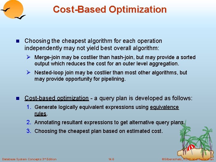
Cost-Based Optimization n Choosing the cheapest algorithm for each operation independently may not yield best overall algorithm: Ø Merge-join may be costlier than hash-join, but may provide a sorted output which reduces the cost for an outer level aggregation. Ø Nested-loop join may be costlier than most other algorithms, but may provide opportunity for pipelining. n Cost-based optimization - a query plan is developed as follows: 1. Generate logically equivalent expressions using equivalence rules. 2. Annotating resultant expressions to get alternative query plans. 3. Choosing the cheapest plan based on estimated cost. Database System Concepts 3 rd Edition 14. 6 ©Silberschatz, Korth and Sudarshan

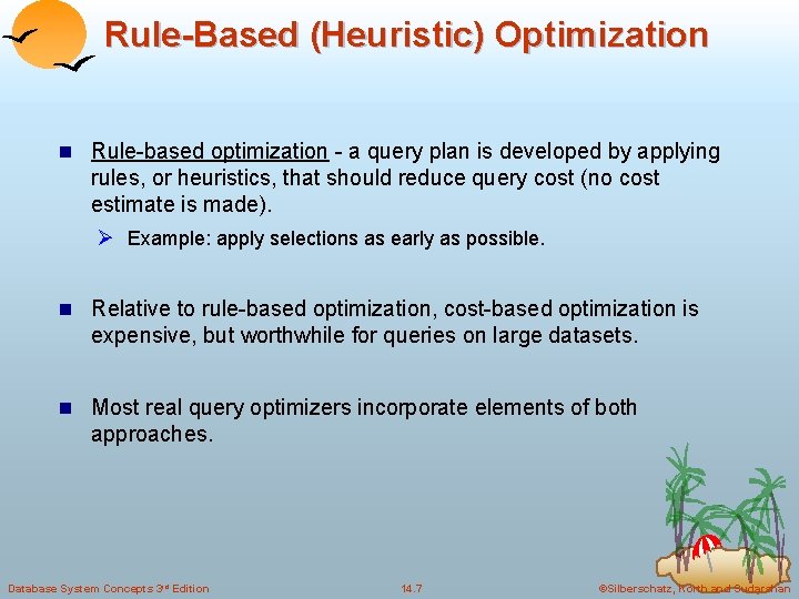
Rule-Based (Heuristic) Optimization n Rule-based optimization - a query plan is developed by applying rules, or heuristics, that should reduce query cost (no cost estimate is made). Ø Example: apply selections as early as possible. n Relative to rule-based optimization, cost-based optimization is expensive, but worthwhile for queries on large datasets. n Most real query optimizers incorporate elements of both approaches. Database System Concepts 3 rd Edition 14. 7 ©Silberschatz, Korth and Sudarshan

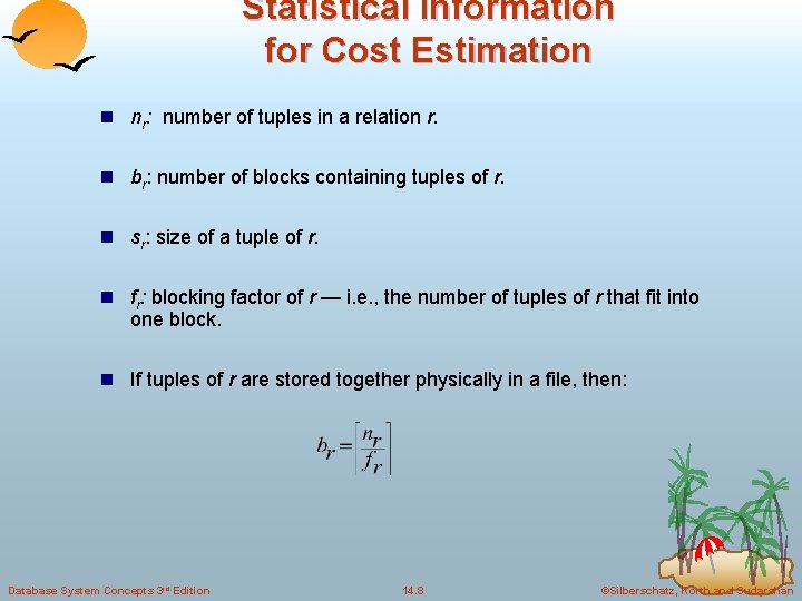
Statistical Information for Cost Estimation n nr: number of tuples in a relation r. n br: number of blocks containing tuples of r. n sr: size of a tuple of r. n fr: blocking factor of r — i. e. , the number of tuples of r that fit into one block. n If tuples of r are stored together physically in a file, then: Database System Concepts 3 rd Edition 14. 8 ©Silberschatz, Korth and Sudarshan

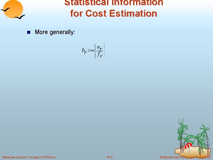
Statistical Information for Cost Estimation n More generally: Database System Concepts 3 rd Edition 14. 9 ©Silberschatz, Korth and Sudarshan

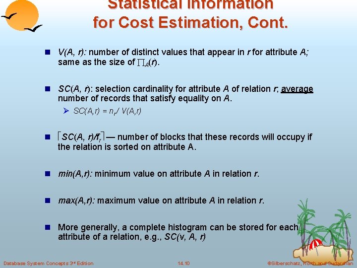
Statistical Information for Cost Estimation, Cont. n V(A, r): number of distinct values that appear in r for attribute A; same as the size of A(r). n SC(A, r): selection cardinality for attribute A of relation r; average number of records that satisfy equality on A. Ø SC(A, r) = nr / V(A, r) n SC(A, r)/fr — number of blocks that these records will occupy if the relation is sorted on attribute A. n min(A, r): minimum value on attribute A in relation r. n max(A, r): maximum value on attribute A in relation r. n More generally, a complete histogram can be stored for each attribute of a relation, e. g. , SC(v, A, r) Database System Concepts 3 rd Edition 14. 10 ©Silberschatz, Korth and Sudarshan

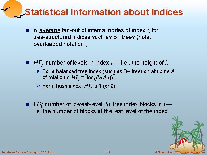
Statistical Information about Indices n fi: average fan-out of internal nodes of index i, for tree-structured indices such as B+ trees (note: overloaded notation!) n HTi: number of levels in index i — i. e. , the height of i. Ø For a balanced tree index (such as B+ tree) on attribute A of relation r, HTi = logfi(V(A, r)). Ø For a hash index, HTi is 1 (or 2) n LBi: number of lowest-level B+ tree index blocks in i — i. e, the number of blocks at the leaf level of the index. Database System Concepts 3 rd Edition 14. 11 ©Silberschatz, Korth and Sudarshan

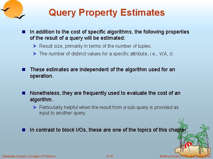
Query Property Estimates n In addition to the cost of specific algorithms, the following properties of the result of a query will be estimated: Ø Result size, primarily in terms of the number of tuples. Ø The number of distinct values for a specific attribute, i. e. , V(A, r). n These estimates are independent of the algorithm used for an operation. n Nonetheless, they are frequently used to evaluate the cost of an algorithm. Ø Particularly helpful when the result from a sub-query is provided as input to another query. n In contrast to block I/Os, these are one of the topics of this chapter. Database System Concepts 3 rd Edition 14. 12 ©Silberschatz, Korth and Sudarshan

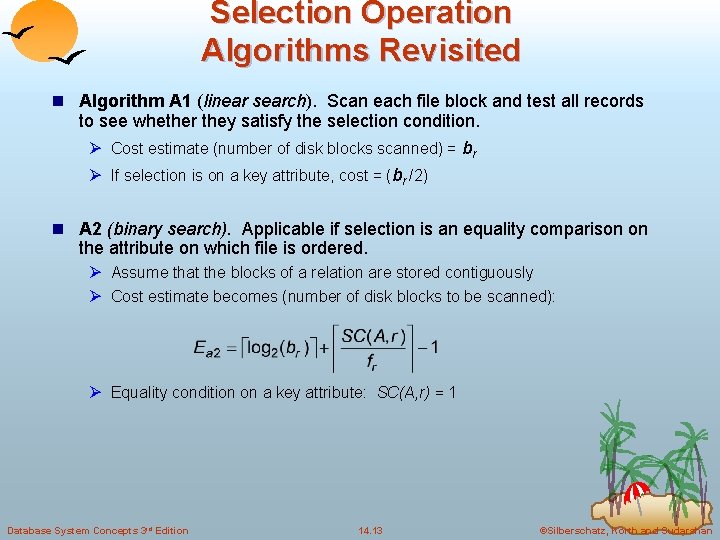
Selection Operation Algorithms Revisited n Algorithm A 1 (linear search). Scan each file block and test all records to see whether they satisfy the selection condition. Ø Cost estimate (number of disk blocks scanned) = br Ø If selection is on a key attribute, cost = (br /2) n A 2 (binary search). Applicable if selection is an equality comparison on the attribute on which file is ordered. Ø Assume that the blocks of a relation are stored contiguously Ø Cost estimate becomes (number of disk blocks to be scanned): Ø Equality condition on a key attribute: SC(A, r) = 1 Database System Concepts 3 rd Edition 14. 13 ©Silberschatz, Korth and Sudarshan

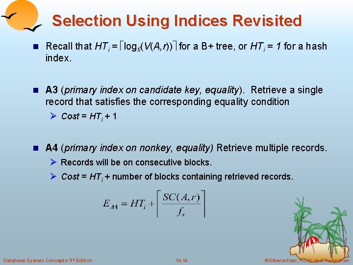
Selection Using Indices Revisited n Recall that HTi = logfi(V(A, r)) for a B+ tree, or HTi = 1 for a hash index. n A 3 (primary index on candidate key, equality). Retrieve a single record that satisfies the corresponding equality condition Ø Cost = HTi + 1 n A 4 (primary index on nonkey, equality) Retrieve multiple records. Ø Records will be on consecutive blocks. Ø Cost = HTi + number of blocks containing retrieved records. Database System Concepts 3 rd Edition 14. 14 ©Silberschatz, Korth and Sudarshan

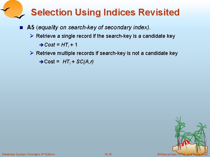
Selection Using Indices Revisited n A 5 (equality on search-key of secondary index). Ø Retrieve a single record if the search-key is a candidate key è Cost = HTi + 1 Ø Retrieve multiple records if search-key is not a candidate key è Cost = HTi + SC(A, r) Database System Concepts 3 rd Edition 14. 15 ©Silberschatz, Korth and Sudarshan

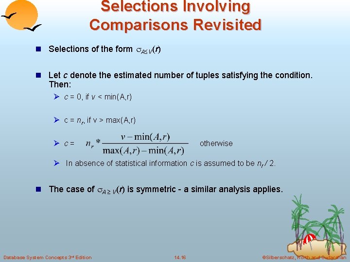
Selections Involving Comparisons Revisited n Selections of the form A V(r) n Let c denote the estimated number of tuples satisfying the condition. Then: Ø c = 0, if v < min(A, r) Ø c = nr, if v > max(A, r) Ø c= otherwise Ø In absence of statistical information c is assumed to be nr / 2. n The case of A V(r) is symmetric - a similar analysis applies. Database System Concepts 3 rd Edition 14. 16 ©Silberschatz, Korth and Sudarshan

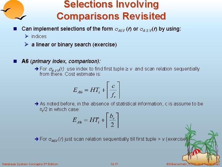
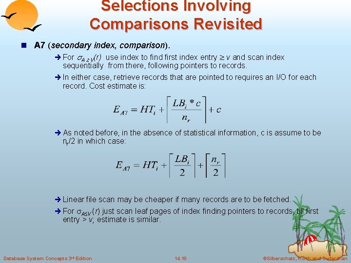
Selections Involving Comparisons Revisited n Can implement selections of the form A V (r) or A V(r) by using: Ø indices Ø a linear or binary search (exercise) n A 6 (primary index, comparison): è For A V(r) use index to find first tuple v and scan relation sequentially from there. Cost estimate is: è As noted before, in the absence of statistical information, c is assume to be nr/2 in which case: è For A V (r) just scan relation sequentially till first tuple > v (exercise) Database System Concepts 3 rd Edition 14. 17 ©Silberschatz, Korth and Sudarshan

Selections Involving Comparisons Revisited n A 7 (secondary index, comparison). è For A V(r) use index to find first index entry v and scan index sequentially from there, following pointers to records. è In either case, retrieve records that are pointed to requires an I/O for each record. Cost estimate is: è As noted before, in the absence of statistical information, c is assume to be nr/2 in which case: è Linear file scan may be cheaper if many records are to be fetched. è For A V (r) just scan leaf pages of index finding pointers to records, till first entry > v; estimate is similar. Database System Concepts 3 rd Edition 14. 18 ©Silberschatz, Korth and Sudarshan

Complex Selections Revisited n Cost estimates for complex selections follow directly from the estimates for A 1 through A 7 n Conjunction: 1 2. . . n(r) Ø A 8 (conjunctive selection using one index). Ø A 9 (conjunctive selection using multiple-key index). Ø A 10 (conjunctive selection by intersection of identifiers). n Disjunction: 1 2 . . . n (r). Ø A 11 (disjunctive selection by union of identifiers). n Negation: Database System Concepts 3 rd Edition (r) 14. 19 ©Silberschatz, Korth and Sudarshan

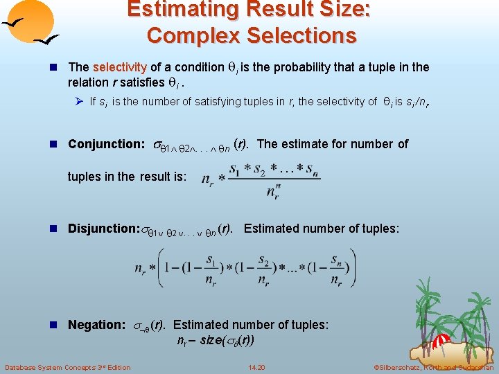
Estimating Result Size: Complex Selections n The selectivity of a condition i is the probability that a tuple in the relation r satisfies i. Ø If si is the number of satisfying tuples in r, the selectivity of i is si /nr. n Conjunction: 1 2. . . n (r). The estimate for number of tuples in the result is: n Disjunction: 1 2 . . . n (r). Estimated number of tuples: n Negation: (r). Estimated number of tuples: nr – size( (r)) Database System Concepts 3 rd Edition 14. 20 ©Silberschatz, Korth and Sudarshan

Transformation of Relational Expressions n Two relational algebra expressions are said to be equivalent if the two expressions generate the same set of tuples in every legal database instance. n Note the order of tuples is considered irrelevant in this context. Ø Question: what about sorting? n An equivalence rule asserts that two expressions are equivalent. Database System Concepts 3 rd Edition 14. 21 ©Silberschatz, Korth and Sudarshan

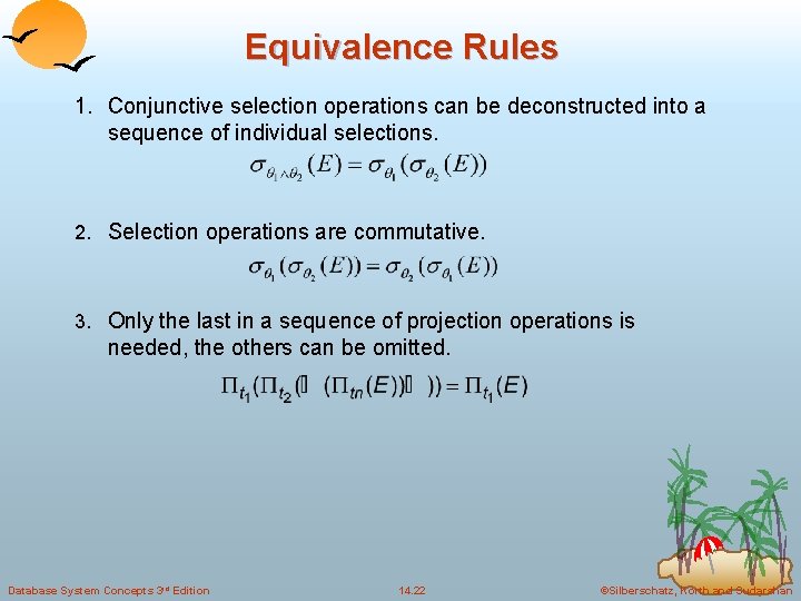
Equivalence Rules 1. Conjunctive selection operations can be deconstructed into a sequence of individual selections. 2. Selection operations are commutative. 3. Only the last in a sequence of projection operations is needed, the others can be omitted. Database System Concepts 3 rd Edition 14. 22 ©Silberschatz, Korth and Sudarshan

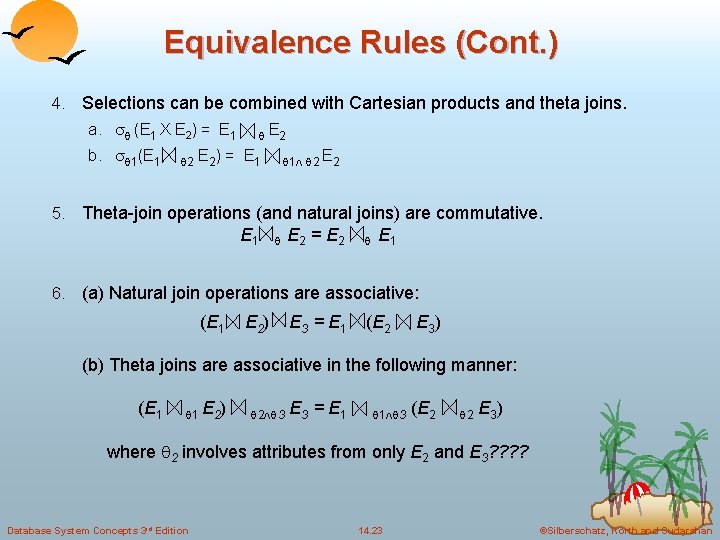
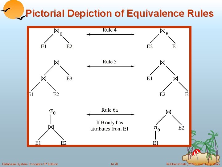
Equivalence Rules (Cont. ) 4. Selections can be combined with Cartesian products and theta joins. a. (E 1 X E 2) = E 1 E 2 b. 1(E 1 2 E 2) = E 1 1 2 E 2 5. Theta-join operations (and natural joins) are commutative. E 1 E 2 = E 2 E 1 6. (a) Natural join operations are associative: (E 1 E 2) E 3 = E 1 (E 2 E 3) (b) Theta joins are associative in the following manner: (E 1 1 E 2) 2 3 E 3 = E 1 1 3 (E 2 2 E 3) where 2 involves attributes from only E 2 and E 3? ? Database System Concepts 3 rd Edition 14. 23 ©Silberschatz, Korth and Sudarshan

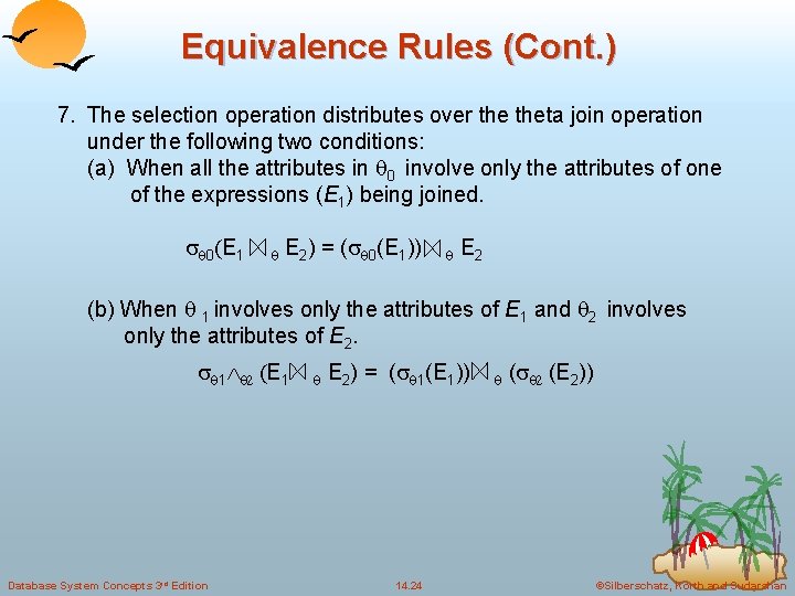
Equivalence Rules (Cont. ) 7. The selection operation distributes over theta join operation under the following two conditions: (a) When all the attributes in 0 involve only the attributes of one of the expressions (E 1) being joined. 0 E 1 E 2) = ( 0(E 1)) E 2 (b) When 1 involves only the attributes of E 1 and 2 involves only the attributes of E 2. 1 E 1 Database System Concepts 3 rd Edition E 2) = ( 1(E 1)) 14. 24 ( (E 2)) ©Silberschatz, Korth and Sudarshan

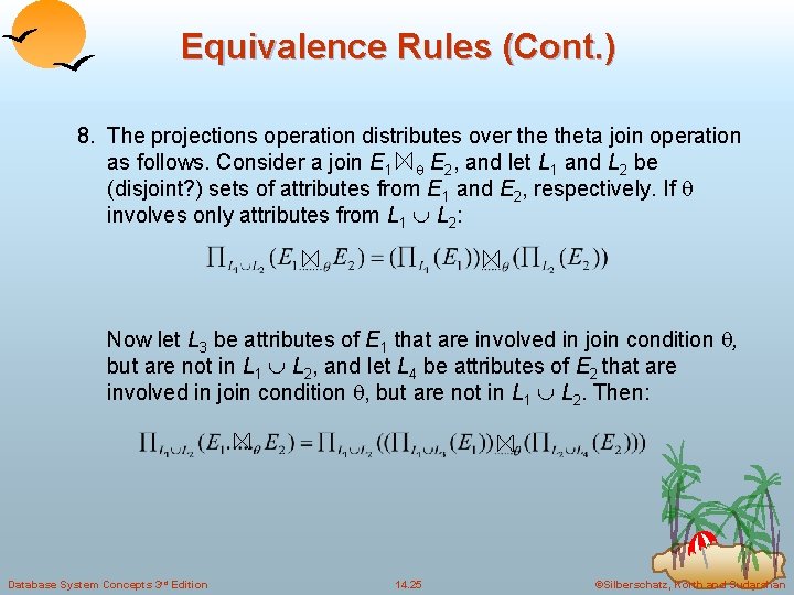
Equivalence Rules (Cont. ) 8. The projections operation distributes over theta join operation as follows. Consider a join E 1 E 2, and let L 1 and L 2 be (disjoint? ) sets of attributes from E 1 and E 2, respectively. If involves only attributes from L 1 L 2: Now let L 3 be attributes of E 1 that are involved in join condition , but are not in L 1 L 2, and let L 4 be attributes of E 2 that are involved in join condition , but are not in L 1 L 2. Then: Database System Concepts 3 rd Edition 14. 25 ©Silberschatz, Korth and Sudarshan

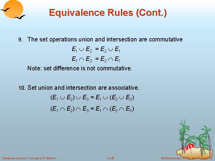
Equivalence Rules (Cont. ) 9. The set operations union and intersection are commutative E 1 E 2 = E 2 E 1 Note: set difference is not commutative. 10. Set union and intersection are associative. (E 1 E 2) E 3 = E 1 (E 2 E 3) Database System Concepts 3 rd Edition 14. 26 ©Silberschatz, Korth and Sudarshan

Equivalence Rules (Cont. ) 11. The selection operation distributes over , and –. (E 1 – E 2) = (E 1) – (E 2) and similarly for and in place of – (E 1 – E 2) = (E 1) – E 2 and similarly for in place of –, but not for 12. The projection operation distributes over union L(E 1 E 2) = ( L(E 1)) ( L(E 2)) Database System Concepts 3 rd Edition 14. 27 ©Silberschatz, Korth and Sudarshan

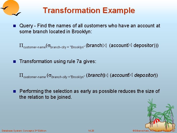
Transformation Example n Query - Find the names of all customers who have an account at some branch located in Brooklyn: customer-name( branch-city = “Brooklyn” (branch (account depositor))) (account depositor)) n Transformation using rule 7 a gives: customer-name ( branch-city =“Brooklyn” (branch) n Performing the selection as early as possible reduces the size of the relation to be joined. Database System Concepts 3 rd Edition 14. 28 ©Silberschatz, Korth and Sudarshan

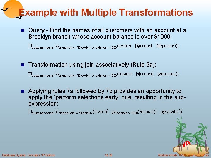
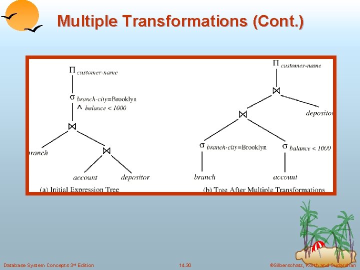
Example with Multiple Transformations n Query - Find the names of all customers with an account at a Brooklyn branch whose account balance is over $1000: customer-name ( branch-city = “Brooklyn” balance > 1000(branch (account depositor))) n Transformation using join associatively (Rule 6 a): customer-name ( branch-city = “Brooklyn” balance > 1000((branch account) depositor)) n Applying rules 7 a followed by 7 b provides an opportunity to apply the “perform selections early” rule, resulting in the subexpression: customer-name (( branch-city = “Brooklyn”(branch) Database System Concepts 3 rd Edition 14. 29 balance > 1000(account)) depositor)) ©Silberschatz, Korth and Sudarshan

Multiple Transformations (Cont. ) Database System Concepts 3 rd Edition 14. 30 ©Silberschatz, Korth and Sudarshan

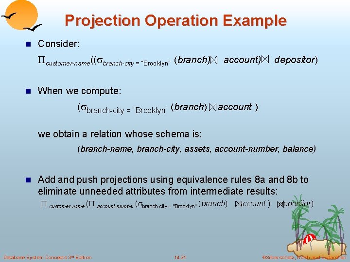
Projection Operation Example n Consider: customer-name(( branch-city = “Brooklyn” (branch) account) depositor) n When we compute: ( branch-city = “Brooklyn” (branch) account ) we obtain a relation whose schema is: (branch-name, branch-city, assets, account-number, balance) n Add and push projections using equivalence rules 8 a and 8 b to eliminate unneeded attributes from intermediate results: customer-name ( account-number ( branch-city = “Brooklyn” (branch) Database System Concepts 3 rd Edition 14. 31 account ) depositor) ©Silberschatz, Korth and Sudarshan

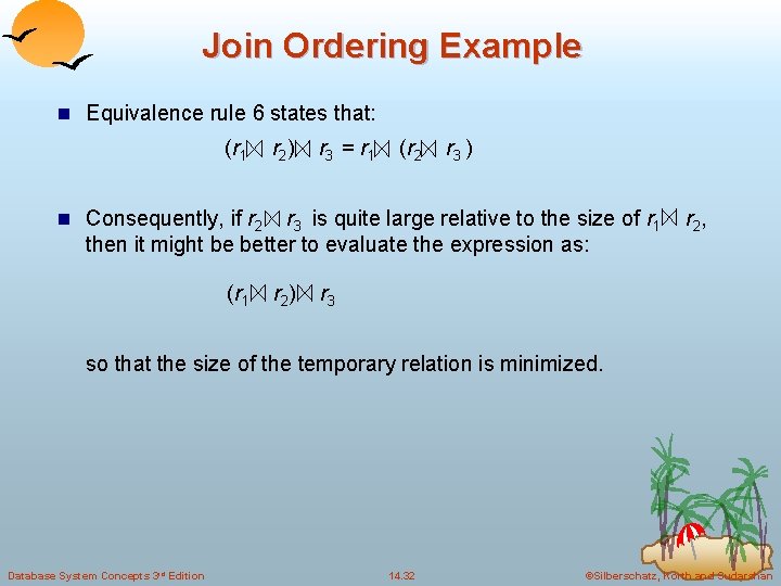
Join Ordering Example n Equivalence rule 6 states that: (r 1 r 2 ) r 3 = r 1 (r 2 r 3 ) n Consequently, if r 2 r 3 is quite large relative to the size of r 1 then it might be better to evaluate the expression as: (r 1 r 2 ) r 2 , r 3 so that the size of the temporary relation is minimized. Database System Concepts 3 rd Edition 14. 32 ©Silberschatz, Korth and Sudarshan

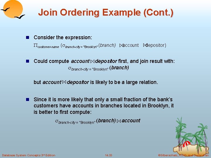
Join Ordering Example (Cont. ) n Consider the expression: customer-name ( branch-city = “Brooklyn” (branch) account depositor) n Could compute account depositor first, and join result with: branch-city = “Brooklyn” (branch) but account depositor is likely to be a large relation. n Since it is more likely that only a small fraction of the bank’s customers have accounts in branches located in Brooklyn, it is better to first compute: branch-city = “Brooklyn” (branch) Database System Concepts 3 rd Edition 14. 33 account ©Silberschatz, Korth and Sudarshan

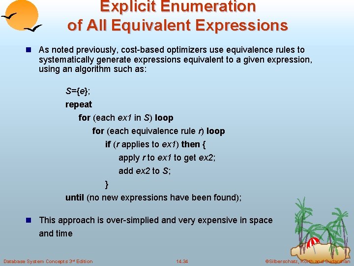
Explicit Enumeration of All Equivalent Expressions n As noted previously, cost-based optimizers use equivalence rules to systematically generate expressions equivalent to a given expression, using an algorithm such as: S={e}; repeat for (each ex 1 in S) loop for (each equivalence rule r) loop if (r applies to ex 1) then { apply r to ex 1 to get ex 2; add ex 2 to S; } until (no new expressions have been found); n This approach is over-simplied and very expensive in space and time Database System Concepts 3 rd Edition 14. 34 ©Silberschatz, Korth and Sudarshan

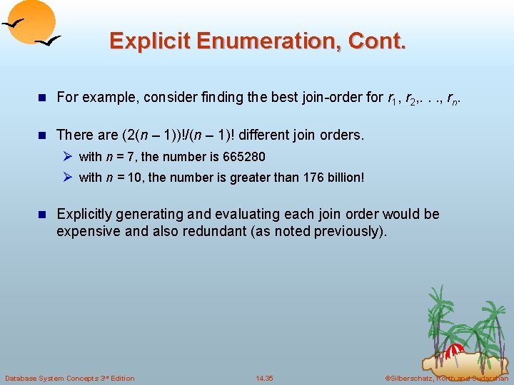
Explicit Enumeration, Cont. n For example, consider finding the best join-order for r 1, r 2, . . . , rn. n There are (2(n – 1))!/(n – 1)! different join orders. Ø with n = 7, the number is 665280 Ø with n = 10, the number is greater than 176 billion! n Explicitly generating and evaluating each join order would be expensive and also redundant (as noted previously). Database System Concepts 3 rd Edition 14. 35 ©Silberschatz, Korth and Sudarshan

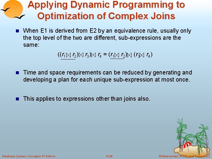
Applying Dynamic Programming to Optimization of Complex Joins n When E 1 is derived from E 2 by an equivalence rule, usually only the top level of the two are different, sub-expressions are the same: ((r 1 r 2 ) r 3 ) r 4 = (r 1 r 2 ) (r 3 r 4 ) n Time and space requirements can be reduced by generating and developing a plan for each unique sub-expression at most once. n This applies to expressions other than joins also. Database System Concepts 3 rd Edition 14. 36 ©Silberschatz, Korth and Sudarshan

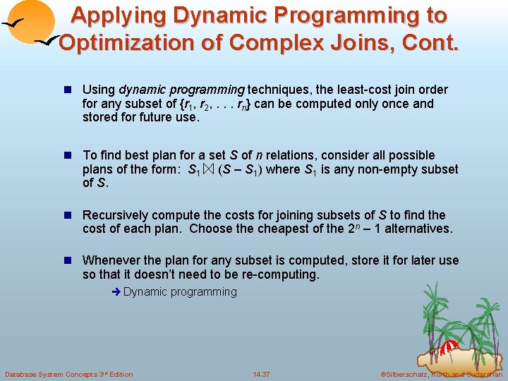
Applying Dynamic Programming to Optimization of Complex Joins, Cont. n Using dynamic programming techniques, the least-cost join order for any subset of {r 1, r 2, . . . rn} can be computed only once and stored for future use. n To find best plan for a set S of n relations, consider all possible plans of the form: S 1 of S. (S – S 1) where S 1 is any non-empty subset n Recursively compute the costs for joining subsets of S to find the cost of each plan. Choose the cheapest of the 2 n – 1 alternatives. n Whenever the plan for any subset is computed, store it for later use so that it doesn’t need to be re-computing. è Dynamic programming Database System Concepts 3 rd Edition 14. 37 ©Silberschatz, Korth and Sudarshan

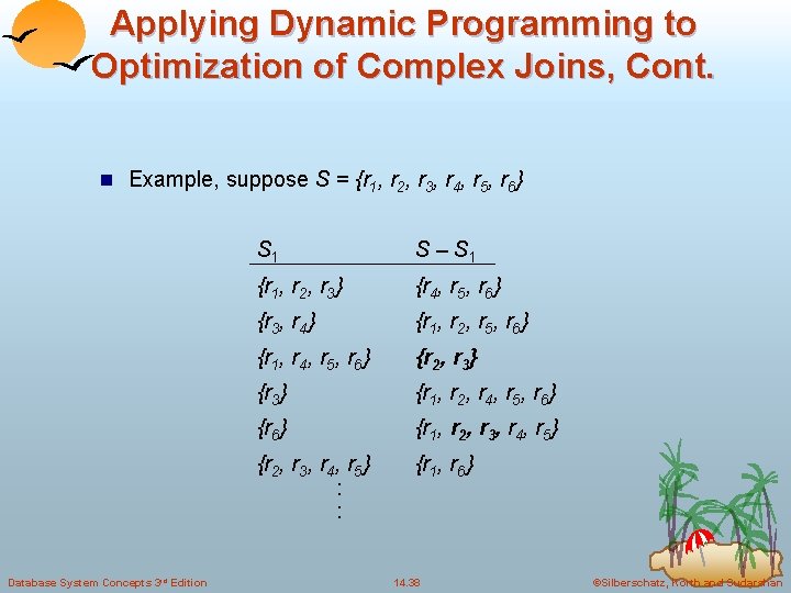
Applying Dynamic Programming to Optimization of Complex Joins, Cont. n Example, suppose S = {r 1, r 2, r 3, r 4, r 5, r 6} Database System Concepts 3 rd Edition S 1 S – S 1 {r 1, r 2, r 3} {r 4, r 5, r 6} {r 3, r 4} {r 1, r 2, r 5, r 6} {r 1, r 4, r 5, r 6} {r 2, r 3} {r 1, r 2, r 4, r 5, r 6} {r 1, r 2, r 3, r 4, r 5} {r 2, r 3, r 4, r 5} : : {r 1, r 6} 14. 38 ©Silberschatz, Korth and Sudarshan

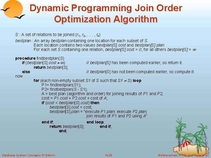
Dynamic Programming Join Order Optimization Algorithm S : A set of relations to be joined {r 1, r 2, . . . , rn} bestplan : An array bestplan containing one location for each subset of S. Each location contains two values bestplan[S]. cost and bestplan[S]. plan For each set S containing one relation, bestplan[S]. cost = 0, for all others bestplan[S] = procedure findbestplan(S) if (bestplan[S]. cost ) // bestplan[S] has been computed earlier, so return it return bestplan[S]; else // bestplan[S] has not been computed earlier, so compute it now for (each non-empty subset S 1 of S such that S 1 S) loop P 1= findbestplan(S 1); P 2= findbestplan(S - S 1); A = best plan (algorithm and order) for joining results of P 1 and P 2; cost = P 1. cost + P 2. cost + cost of A; if (cost < bestplan[S]. cost) then bestplan[S]. cost = cost; bestplan[S]. plan = “execute P 1. plan; execute P 2. plan; join results of P 1 and P 2 using A” end if; end loop; return bestplan[S]; end if; end; Database System Concepts 3 rd Edition 14. 39 ©Silberschatz, Korth and Sudarshan

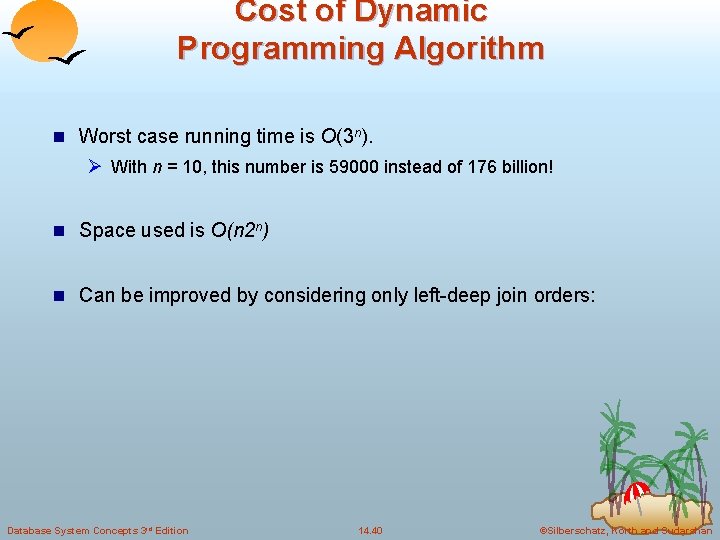
Cost of Dynamic Programming Algorithm n Worst case running time is O(3 n). Ø With n = 10, this number is 59000 instead of 176 billion! n Space used is O(n 2 n) n Can be improved by considering only left-deep join orders: Database System Concepts 3 rd Edition 14. 40 ©Silberschatz, Korth and Sudarshan

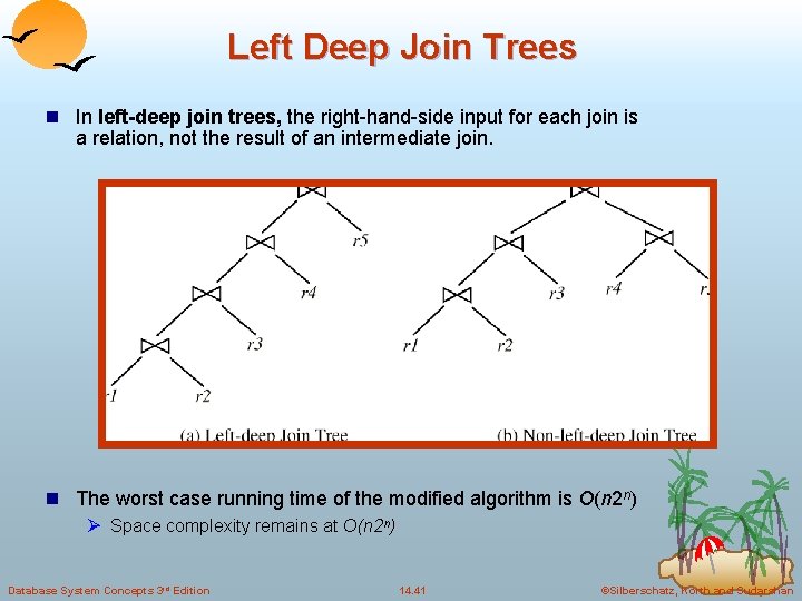
Left Deep Join Trees n In left-deep join trees, the right-hand-side input for each join is a relation, not the result of an intermediate join. n The worst case running time of the modified algorithm is O(n 2 n) Ø Space complexity remains at O(n 2 n) Database System Concepts 3 rd Edition 14. 41 ©Silberschatz, Korth and Sudarshan

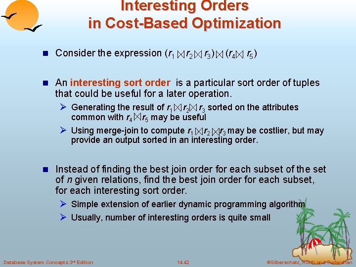
Interesting Orders in Cost-Based Optimization n Consider the expression (r 1 r 2 r 3 ) (r 4 r 5 ) n An interesting sort order is a particular sort order of tuples that could be useful for a later operation. Ø Generating the result of r 1 r 2 r 3 sorted on the attributes common with r 4 r 5 may be useful Ø Using merge-join to compute r 1 r 2 r 3 may be costlier, but may provide an output sorted in an interesting order. n Instead of finding the best join order for each subset of the set of n given relations, find the best join order for each subset, for each interesting sort order. Ø Simple extension of earlier dynamic programming algorithm Ø Usually, number of interesting orders is quite small Database System Concepts 3 rd Edition 14. 42 ©Silberschatz, Korth and Sudarshan

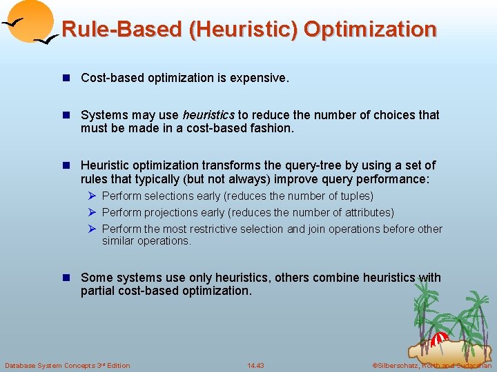
Rule-Based (Heuristic) Optimization n Cost-based optimization is expensive. n Systems may use heuristics to reduce the number of choices that must be made in a cost-based fashion. n Heuristic optimization transforms the query-tree by using a set of rules that typically (but not always) improve query performance: Ø Perform selections early (reduces the number of tuples) Ø Perform projections early (reduces the number of attributes) Ø Perform the most restrictive selection and join operations before other similar operations. n Some systems use only heuristics, others combine heuristics with partial cost-based optimization. Database System Concepts 3 rd Edition 14. 43 ©Silberschatz, Korth and Sudarshan

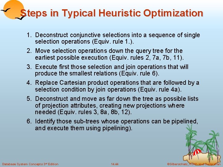
Steps in Typical Heuristic Optimization 1. Deconstruct conjunctive selections into a sequence of single selection operations (Equiv. rule 1. ). 2. Move selection operations down the query tree for the earliest possible execution (Equiv. rules 2, 7 a, 7 b, 11). 3. Execute first those selection and join operations that will produce the smallest relations (Equiv. rule 6). 4. Replace Cartesian product operations that are followed by a selection condition by join operations (Equiv. rule 4 a). 5. Deconstruct and move as far down the tree as possible lists of projection attributes, creating new projections where needed (Equiv. rules 3, 8 a, 8 b, 12). 6. Identify those sub-trees whose operations can be pipelined, and execute them using pipelining). Database System Concepts 3 rd Edition 14. 44 ©Silberschatz, Korth and Sudarshan

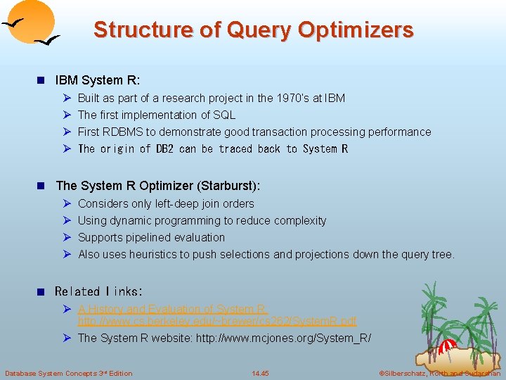
Structure of Query Optimizers n IBM System R: Ø Built as part of a research project in the 1970’s at IBM Ø The first implementation of SQL Ø First RDBMS to demonstrate good transaction processing performance Ø The origin of DB 2 can be traced back to System R n The System R Optimizer (Starburst): Ø Considers only left-deep join orders Ø Using dynamic programming to reduce complexity Ø Supports pipelined evaluation Ø Also uses heuristics to push selections and projections down the query tree. n Related Links: Ø A History and Evaluation of System R: http: //www. cs. berkeley. edu/~brewer/cs 262/System. R. pdf Ø The System R website: http: //www. mcjones. org/System_R/ Database System Concepts 3 rd Edition 14. 45 ©Silberschatz, Korth and Sudarshan

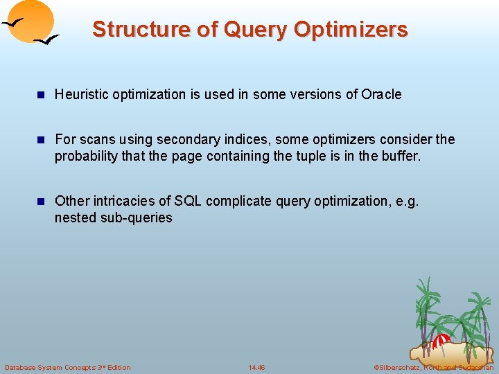
Structure of Query Optimizers n Heuristic optimization is used in some versions of Oracle n For scans using secondary indices, some optimizers consider the probability that the page containing the tuple is in the buffer. n Other intricacies of SQL complicate query optimization, e. g. nested sub-queries Database System Concepts 3 rd Edition 14. 46 ©Silberschatz, Korth and Sudarshan

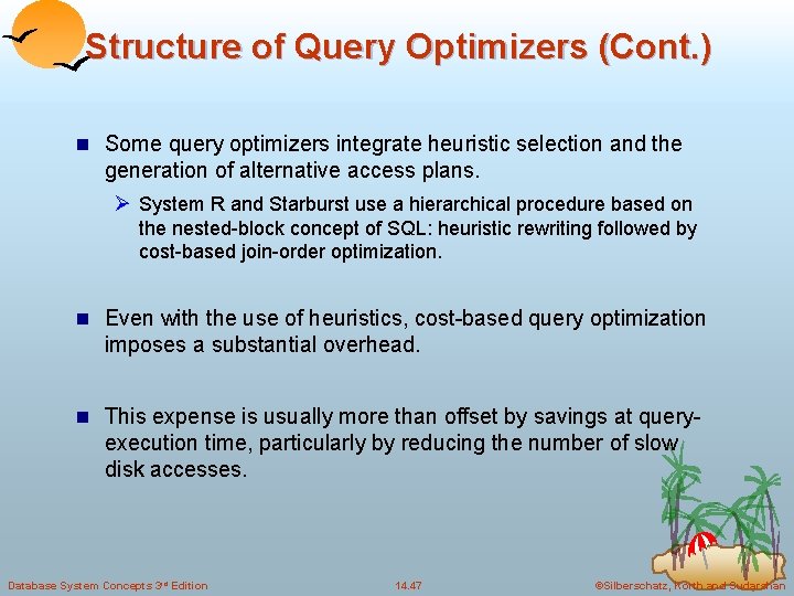
Structure of Query Optimizers (Cont. ) n Some query optimizers integrate heuristic selection and the generation of alternative access plans. Ø System R and Starburst use a hierarchical procedure based on the nested-block concept of SQL: heuristic rewriting followed by cost-based join-order optimization. n Even with the use of heuristics, cost-based query optimization imposes a substantial overhead. n This expense is usually more than offset by savings at query- execution time, particularly by reducing the number of slow disk accesses. Database System Concepts 3 rd Edition 14. 47 ©Silberschatz, Korth and Sudarshan

End of Chapter (Extra slides with details of selection cost estimation follow)

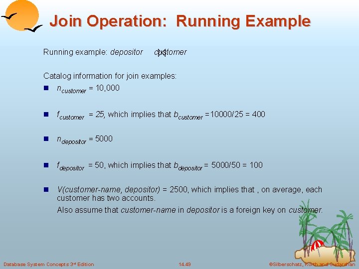
Join Operation: Running Example Running example: depositor customer Catalog information for join examples: n ncustomer = 10, 000 n fcustomer = 25, which implies that bcustomer =10000/25 = 400 n ndepositor = 5000 n fdepositor = 50, which implies that bdepositor = 5000/50 = 100 n V(customer-name, depositor) = 2500, which implies that , on average, each customer has two accounts. Also assume that customer-name in depositor is a foreign key on customer. Database System Concepts 3 rd Edition 14. 49 ©Silberschatz, Korth and Sudarshan

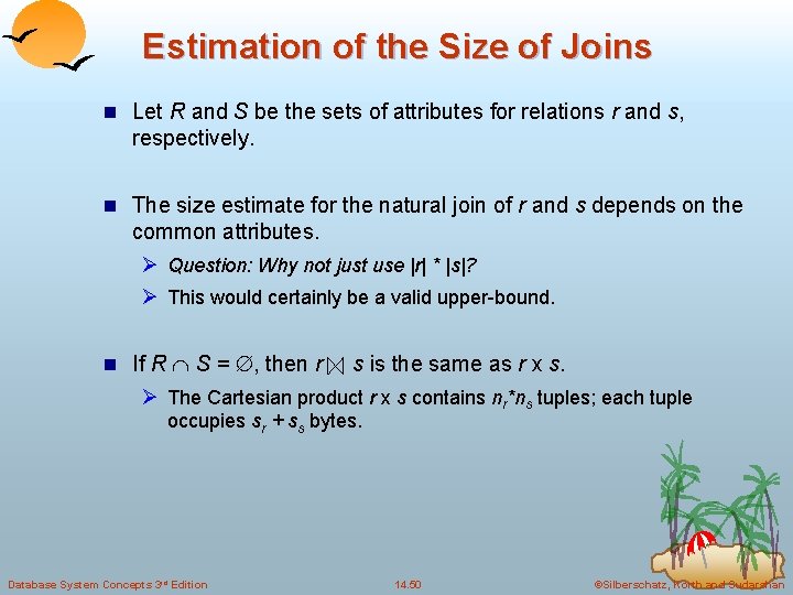
Estimation of the Size of Joins n Let R and S be the sets of attributes for relations r and s, respectively. n The size estimate for the natural join of r and s depends on the common attributes. Ø Question: Why not just use |r| * |s|? Ø This would certainly be a valid upper-bound. n If R S = , then r s is the same as r x s. Ø The Cartesian product r x s contains nr*ns tuples; each tuple occupies sr + ss bytes. Database System Concepts 3 rd Edition 14. 50 ©Silberschatz, Korth and Sudarshan

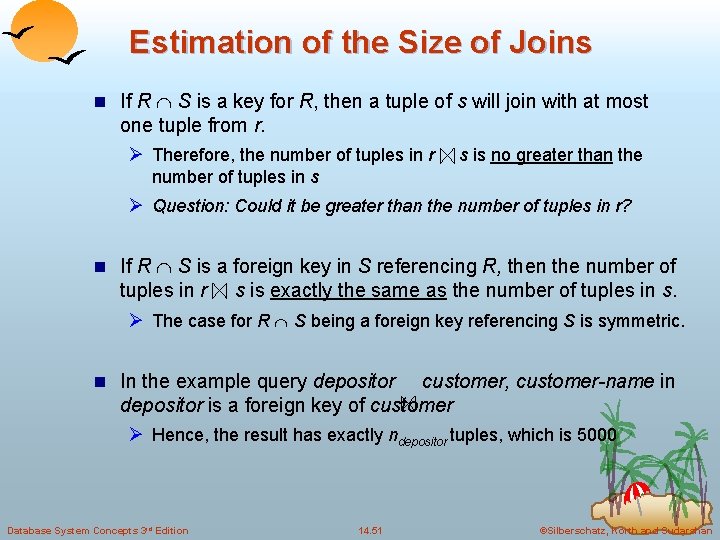
Estimation of the Size of Joins n If R S is a key for R, then a tuple of s will join with at most one tuple from r. Ø Therefore, the number of tuples in r s is no greater than the number of tuples in s Ø Question: Could it be greater than the number of tuples in r? n If R S is a foreign key in S referencing R, then the number of tuples in r s is exactly the same as the number of tuples in s. Ø The case for R S being a foreign key referencing S is symmetric. n In the example query depositor customer, customer-name in depositor is a foreign key of customer Ø Hence, the result has exactly ndepositor tuples, which is 5000 Database System Concepts 3 rd Edition 14. 51 ©Silberschatz, Korth and Sudarshan

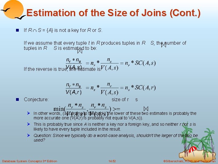
Estimation of the Size of Joins (Cont. ) n If R S = {A} is not a key for R or S. If we assume that every tuple t in R produces tuples in R S is estimated to be: S, the number of If the reverse is true, the estimate is: n Conjecture: size of r s Ø In other words, (according to the book) the lower of these two estimates is probably the more accurate one (V(A, r) is probably not equal to V(A, s)). Ø This is probably true since A is neither a key nor a foreign key, and so neither r nor s is likely to have every tuple included in the result. Ø Question: Since we typically do a worst-case analysis, shouldn’t the larger of the two be used? Database System Concepts 3 rd Edition 14. 52 ©Silberschatz, Korth and Sudarshan

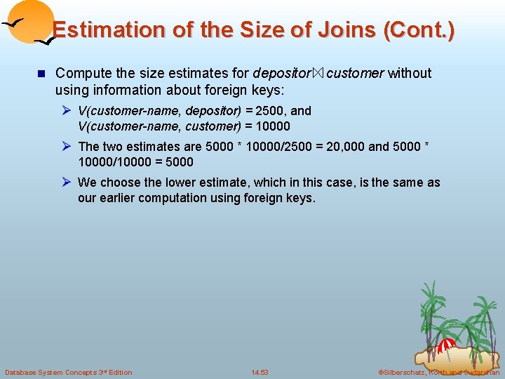
Estimation of the Size of Joins (Cont. ) n Compute the size estimates for depositor customer without using information about foreign keys: Ø V(customer-name, depositor) = 2500, and V(customer-name, customer) = 10000 Ø The two estimates are 5000 * 10000/2500 = 20, 000 and 5000 * 10000/10000 = 5000 Ø We choose the lower estimate, which in this case, is the same as our earlier computation using foreign keys. Database System Concepts 3 rd Edition 14. 53 ©Silberschatz, Korth and Sudarshan

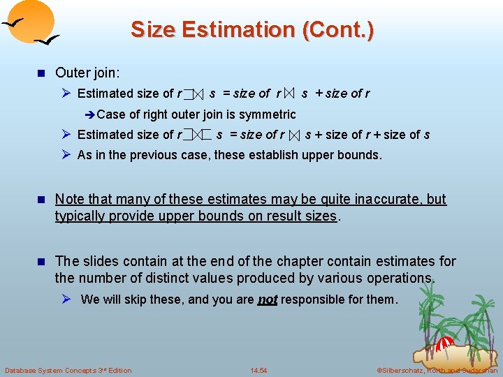
Size Estimation (Cont. ) n Outer join: Ø Estimated size of r s = size of r s + size of r è Case of right outer join is symmetric Ø Estimated size of r s = size of r s + size of r + size of s Ø As in the previous case, these establish upper bounds. n Note that many of these estimates may be quite inaccurate, but typically provide upper bounds on result sizes. n The slides contain at the end of the chapter contain estimates for the number of distinct values produced by various operations. Ø We will skip these, and you are not responsible for them. Database System Concepts 3 rd Edition 14. 54 ©Silberschatz, Korth and Sudarshan

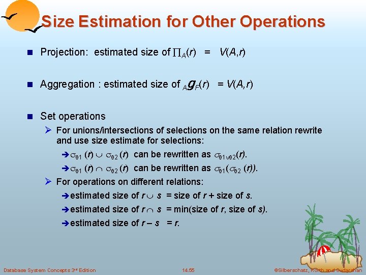
Size Estimation for Other Operations n Projection: estimated size of A(r) = V(A, r) n Aggregation : estimated size of g. F(r) A = V(A, r) n Set operations Ø For unions/intersections of selections on the same relation rewrite and use size estimate for selections: è 1 (r) 2 (r) can be rewritten as 1 2(r). è 1 (r) 2 (r) can be rewritten as 1( 2 (r)). Ø For operations on different relations: è estimated size of r s = size of r + size of s. è estimated size of r s = min(size of r, size of s). è estimated size of r – s = r. Database System Concepts 3 rd Edition 14. 55 ©Silberschatz, Korth and Sudarshan

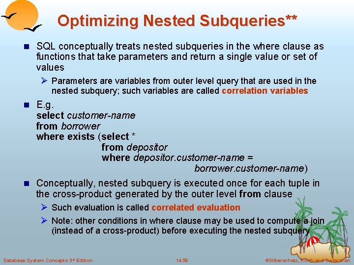
Optimizing Nested Subqueries** n SQL conceptually treats nested subqueries in the where clause as functions that take parameters and return a single value or set of values Ø Parameters are variables from outer level query that are used in the nested subquery; such variables are called correlation variables n E. g. select customer-name from borrower where exists (select * from depositor where depositor. customer-name = borrower. customer-name) n Conceptually, nested subquery is executed once for each tuple in the cross-product generated by the outer level from clause Ø Such evaluation is called correlated evaluation Ø Note: other conditions in where clause may be used to compute a join (instead of a cross-product) before executing the nested subquery Database System Concepts 3 rd Edition 14. 56 ©Silberschatz, Korth and Sudarshan

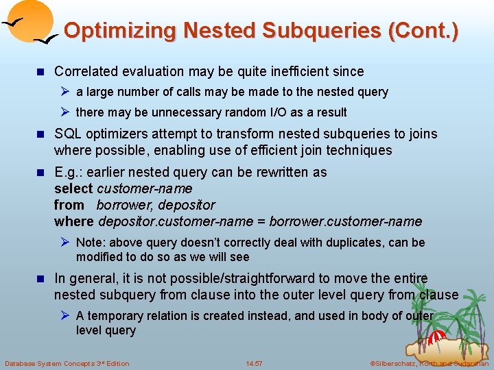
Optimizing Nested Subqueries (Cont. ) n Correlated evaluation may be quite inefficient since Ø a large number of calls may be made to the nested query Ø there may be unnecessary random I/O as a result n SQL optimizers attempt to transform nested subqueries to joins where possible, enabling use of efficient join techniques n E. g. : earlier nested query can be rewritten as select customer-name from borrower, depositor where depositor. customer-name = borrower. customer-name Ø Note: above query doesn’t correctly deal with duplicates, can be modified to do so as we will see n In general, it is not possible/straightforward to move the entire nested subquery from clause into the outer level query from clause Ø A temporary relation is created instead, and used in body of outer level query Database System Concepts 3 rd Edition 14. 57 ©Silberschatz, Korth and Sudarshan

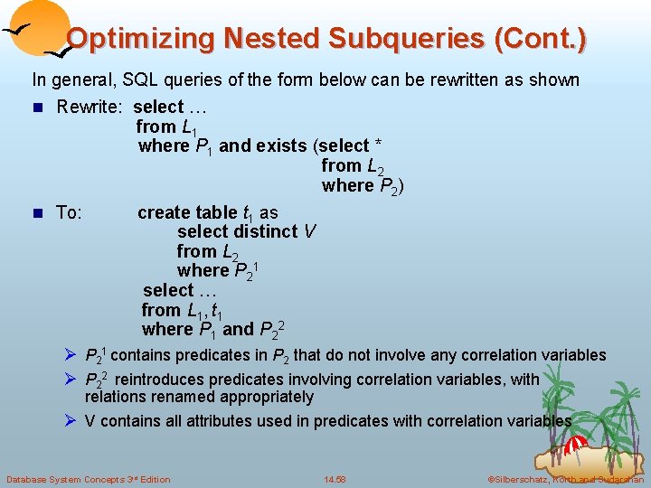
Optimizing Nested Subqueries (Cont. ) In general, SQL queries of the form below can be rewritten as shown n Rewrite: select … from L 1 where P 1 and exists (select * from L 2 where P 2) n To: create table t 1 as select distinct V from L 2 where P 21 select … from L 1, t 1 where P 1 and P 22 Ø P 21 contains predicates in P 2 that do not involve any correlation variables Ø P 22 reintroduces predicates involving correlation variables, with relations renamed appropriately Ø V contains all attributes used in predicates with correlation variables Database System Concepts 3 rd Edition 14. 58 ©Silberschatz, Korth and Sudarshan

Optimizing Nested Subqueries (Cont. ) n In our example, the original nested query would be transformed to create table t 1 as select distinct customer-name from depositor select customer-name from borrower, t 1 where t 1. customer-name = borrower. customer-name n The process of replacing a nested query by a query with a join (possibly with a temporary relation) is called decorrelation. n Decorrelation is more complicated when Ø the nested subquery uses aggregation, or Ø when the result of the nested subquery is used to test for equality, or Ø when the condition linking the nested subquery to the other query is not exists, Ø and so on. Database System Concepts 3 rd Edition 14. 59 ©Silberschatz, Korth and Sudarshan

Materialized Views** n A materialized view is a view whose contents are computed and stored. n Consider the view create view branch-total-loan(branch-name, total-loan) as select branch-name, sum(amount) from loan groupby branch-name n Materializing the above view would be very useful if the total loan amount is required frequently Ø Saves the effort of finding multiple tuples and adding up their amounts Database System Concepts 3 rd Edition 14. 60 ©Silberschatz, Korth and Sudarshan

Materialized View Maintenance n The task of keeping a materialized view up-to-date with the underlying data is known as materialized view maintenance n Materialized views can be maintained by recomputation on every update n A better option is to use incremental view maintenance Ø Changes to database relations are used to compute changes to materialized view, which is then updated n View maintenance can be done by Ø Manually defining triggers on insert, delete, and update of each relation in the view definition Ø Manually written code to update the view whenever database relations are updated Ø Supported directly by the database Database System Concepts 3 rd Edition 14. 61 ©Silberschatz, Korth and Sudarshan

Incremental View Maintenance n The changes (inserts and deletes) to a relation or expressions are referred to as its differential Ø Set of tuples inserted to and deleted from r are denoted ir and dr n To simplify our description, we only consider inserts and deletes Ø We replace updates to a tuple by deletion of the tuple followed by insertion of the update tuple n We describe how to compute the change to the result of each relational operation, given changes to its inputs n We then outline how to handle relational algebra expressions Database System Concepts 3 rd Edition 14. 62 ©Silberschatz, Korth and Sudarshan

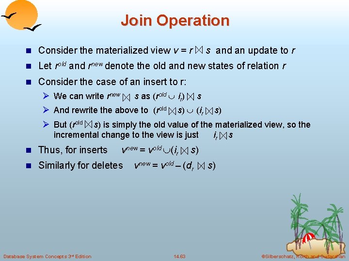
Join Operation n Consider the materialized view v = r s and an update to r n Let rold and rnew denote the old and new states of relation r n Consider the case of an insert to r: s as (rold ir) Ø We can write rnew Ø And rewrite the above to (rold s s) (ir s) Ø But (rold s) is simply the old value of the materialized view, so the incremental change to the view is just ir s n Thus, for inserts vnew = vold (ir n Similarly for deletes Database System Concepts 3 rd Edition s) vnew = vold – (dr 14. 63 s) ©Silberschatz, Korth and Sudarshan

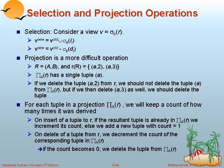
Selection and Projection Operations n Selection: Consider a view v = (r). Ø vnew = vold (ir) Ø vnew = vold - (dr) n Projection is a more difficult operation Ø R = (A, B), and r(R) = { (a, 2), (a, 3)} Ø A(r) has a single tuple (a). Ø If we delete the tuple (a, 2) from r, we should not delete the tuple (a) from A(r), but if we then delete (a, 3) as well, we should delete the tuple n For each tuple in a projection A(r) , we will keep a count of how many times it was derived Ø On insert of a tuple to r, if the resultant tuple is already in A(r) we increment its count, else we add a new tuple with count = 1 Ø On delete of a tuple from r, we decrement the count of the corresponding tuple in A(r) è if the count becomes 0, we delete the tuple from A(r) Database System Concepts 3 rd Edition 14. 64 ©Silberschatz, Korth and Sudarshan

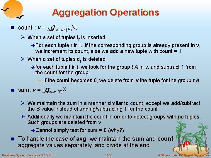
Aggregation Operations n count : v = Agcount(B)(r). Ø When a set of tuples ir is inserted è For each tuple r in ir, if the corresponding group is already present in v, we increment its count, else we add a new tuple with count = 1 Ø When a set of tuples dr is deleted è for each tuple t in ir. we look for the group t. A in v, and subtract 1 from the count for the group. – If the count becomes 0, we delete from v the tuple for the group t. A n sum: v = gsum (B)(r) A Ø We maintain the sum in a manner similar to count, except we add/subtract the B value instead of adding/subtracting 1 for the count Ø Additionally we maintain the count in order to detect groups with no tuples. Such groups are deleted from v è Cannot simply test for sum = 0 (why? ) n To handle the case of avg, we maintain the sum and count aggregate values separately, and divide at the end Database System Concepts 3 rd Edition 14. 65 ©Silberschatz, Korth and Sudarshan

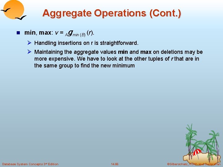
Aggregate Operations (Cont. ) n min, max: v = gmin (B) (r). A Ø Handling insertions on r is straightforward. Ø Maintaining the aggregate values min and max on deletions may be more expensive. We have to look at the other tuples of r that are in the same group to find the new minimum Database System Concepts 3 rd Edition 14. 66 ©Silberschatz, Korth and Sudarshan

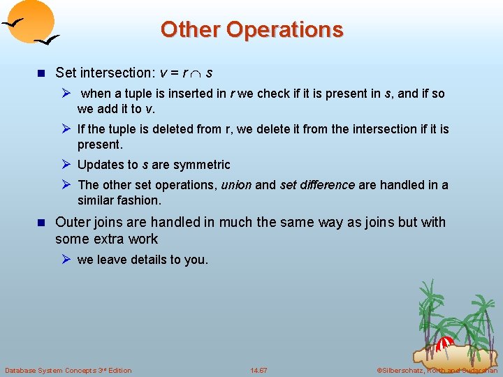
Other Operations n Set intersection: v = r s Ø when a tuple is inserted in r we check if it is present in s, and if so we add it to v. Ø If the tuple is deleted from r, we delete it from the intersection if it is present. Ø Updates to s are symmetric Ø The other set operations, union and set difference are handled in a similar fashion. n Outer joins are handled in much the same way as joins but with some extra work Ø we leave details to you. Database System Concepts 3 rd Edition 14. 67 ©Silberschatz, Korth and Sudarshan

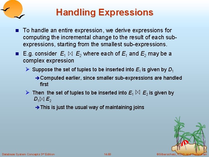
Handling Expressions n To handle an entire expression, we derive expressions for computing the incremental change to the result of each subexpressions, starting from the smallest sub-expressions. n E. g. consider E 1 E 2 where each of E 1 and E 2 may be a complex expression Ø Suppose the set of tuples to be inserted into E 1 is given by D 1 è Computed earlier, since smaller sub-expressions are handled first Ø Then the set of tuples to be inserted into E 1 D 1 E 2 is given by è This is just the usual way of maintaining joins Database System Concepts 3 rd Edition 14. 68 ©Silberschatz, Korth and Sudarshan

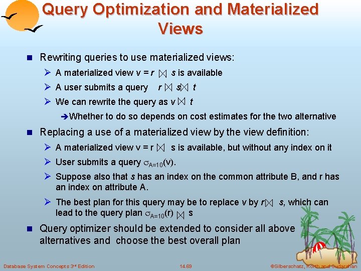
Query Optimization and Materialized Views n Rewriting queries to use materialized views: Ø A materialized view v = r Ø A user submits a query s is available r s Ø We can rewrite the query as v t t è Whether to do so depends on cost estimates for the two alternative n Replacing a use of a materialized view by the view definition: Ø A materialized view v = r s is available, but without any index on it Ø User submits a query A=10(v). Ø Suppose also that s has an index on the common attribute B, and r has an index on attribute A. Ø The best plan for this query may be to replace v by r lead to the query plan A=10(r) s, which can s n Query optimizer should be extended to consider all above alternatives and choose the best overall plan Database System Concepts 3 rd Edition 14. 69 ©Silberschatz, Korth and Sudarshan

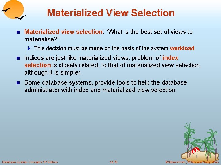
Materialized View Selection n Materialized view selection: “What is the best set of views to materialize? ”. Ø This decision must be made on the basis of the system workload n Indices are just like materialized views, problem of index selection is closely related, to that of materialized view selection, although it is simpler. n Some database systems, provide tools to help the database administrator with index and materialized view selection. Database System Concepts 3 rd Edition 14. 70 ©Silberschatz, Korth and Sudarshan

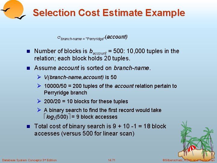
Selection Cost Estimate Example branch-name = “Perryridge”(account) n Number of blocks is baccount = 500: 10, 000 tuples in the relation; each block holds 20 tuples. n Assume account is sorted on branch-name. Ø V(branch-name, account) is 50 Ø 10000/50 = 200 tuples of the account relation pertain to Perryridge branch Ø 200/20 = 10 blocks for these tuples Ø A binary search to find the first record would take log 2(500) = 9 block accesses n Total cost of binary search is 9 + 10 -1 = 18 block accesses (versus 500 for linear scan) Database System Concepts 3 rd Edition 14. 71 ©Silberschatz, Korth and Sudarshan

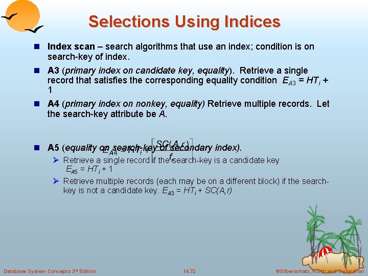
Selections Using Indices n Index scan – search algorithms that use an index; condition is on search-key of index. n A 3 (primary index on candidate key, equality). Retrieve a single record that satisfies the corresponding equality condition EA 3 = HTi + 1 n A 4 (primary index on nonkey, equality) Retrieve multiple records. Let the search-key attribute be A. n A 5 (equality on search-key of secondary index). Ø Retrieve a single record if the search-key is a candidate key EA 5 = HTi + 1 Ø Retrieve multiple records (each may be on a different block) if the searchkey is not a candidate key. EA 3 = HTi + SC(A, r) Database System Concepts 3 rd Edition 14. 72 ©Silberschatz, Korth and Sudarshan

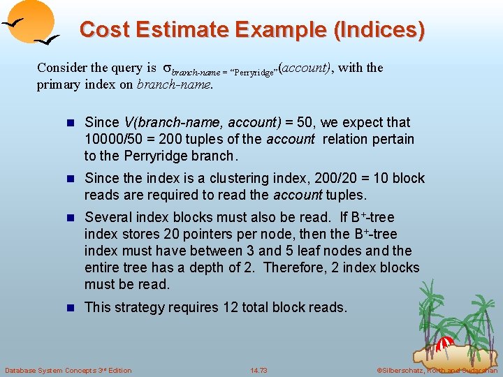
Cost Estimate Example (Indices) Consider the query is branch-name = “Perryridge”(account), with the primary index on branch-name. n Since V(branch-name, account) = 50, we expect that 10000/50 = 200 tuples of the account relation pertain to the Perryridge branch. n Since the index is a clustering index, 200/20 = 10 block reads are required to read the account tuples. n Several index blocks must also be read. If B+-tree index stores 20 pointers per node, then the B+-tree index must have between 3 and 5 leaf nodes and the entire tree has a depth of 2. Therefore, 2 index blocks must be read. n This strategy requires 12 total block reads. Database System Concepts 3 rd Edition 14. 73 ©Silberschatz, Korth and Sudarshan

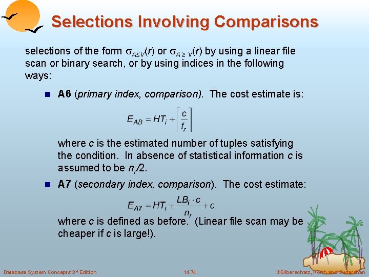
Selections Involving Comparisons selections of the form A V(r) or A V(r) by using a linear file scan or binary search, or by using indices in the following ways: n A 6 (primary index, comparison). The cost estimate is: where c is the estimated number of tuples satisfying the condition. In absence of statistical information c is assumed to be nr/2. n A 7 (secondary index, comparison). The cost estimate: where c is defined as before. (Linear file scan may be cheaper if c is large!). Database System Concepts 3 rd Edition 14. 74 ©Silberschatz, Korth and Sudarshan

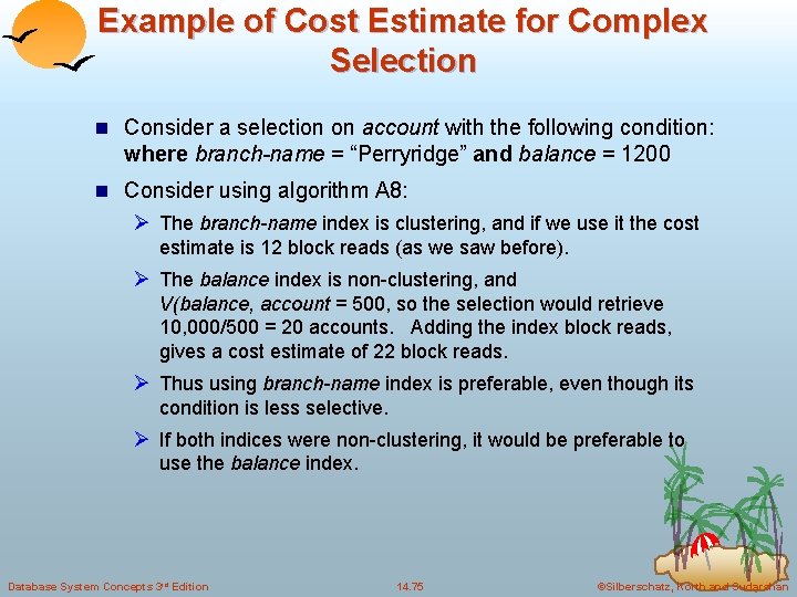
Example of Cost Estimate for Complex Selection n Consider a selection on account with the following condition: where branch-name = “Perryridge” and balance = 1200 n Consider using algorithm A 8: Ø The branch-name index is clustering, and if we use it the cost estimate is 12 block reads (as we saw before). Ø The balance index is non-clustering, and V(balance, account = 500, so the selection would retrieve 10, 000/500 = 20 accounts. Adding the index block reads, gives a cost estimate of 22 block reads. Ø Thus using branch-name index is preferable, even though its condition is less selective. Ø If both indices were non-clustering, it would be preferable to use the balance index. Database System Concepts 3 rd Edition 14. 75 ©Silberschatz, Korth and Sudarshan

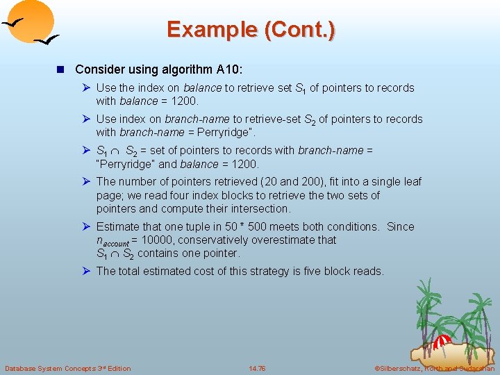
Example (Cont. ) n Consider using algorithm A 10: Ø Use the index on balance to retrieve set S 1 of pointers to records with balance = 1200. Ø Use index on branch-name to retrieve-set S 2 of pointers to records with branch-name = Perryridge”. Ø S 1 S 2 = set of pointers to records with branch-name = “Perryridge” and balance = 1200. Ø The number of pointers retrieved (20 and 200), fit into a single leaf page; we read four index blocks to retrieve the two sets of pointers and compute their intersection. Ø Estimate that one tuple in 50 * 500 meets both conditions. Since naccount = 10000, conservatively overestimate that S 1 S 2 contains one pointer. Ø The total estimated cost of this strategy is five block reads. Database System Concepts 3 rd Edition 14. 76 ©Silberschatz, Korth and Sudarshan

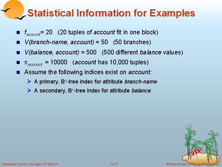
Statistical Information for Examples n faccount= 20 (20 tuples of account fit in one block) n V(branch-name, account) = 50 (50 branches) n V(balance, account) = 500 (500 different balance values) n account = 10000 (account has 10, 000 tuples) n Assume the following indices exist on account: Ø A primary, B+-tree index for attribute branch-name Ø A secondary, B+-tree index for attribute balance Database System Concepts 3 rd Edition 14. 77 ©Silberschatz, Korth and Sudarshan

Pictorial Depiction of Equivalence Rules Database System Concepts 3 rd Edition 14. 78 ©Silberschatz, Korth and Sudarshan

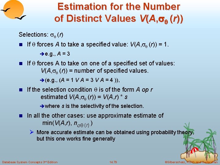
Estimation for the Number of Distinct Values V(A, (r)) Selections: (r) n If forces A to take a specified value: V(A, (r)) = 1. è e. g. , A = 3 n If forces A to take on one of a specified set of values: V(A, (r)) = number of specified values. è (e. g. , (A = 1 V A = 3 V A = 4 )), n If the selection condition is of the form A op r estimated V(A, (r)) = V(A, r) * s è where s is the selectivity of the selection. n In all the other cases: use approximate estimate of min(V(A, r), n (r) ) Ø More accurate estimate can be obtained using probability theory, but this one works fine generally Database System Concepts 3 rd Edition 14. 79 ©Silberschatz, Korth and Sudarshan

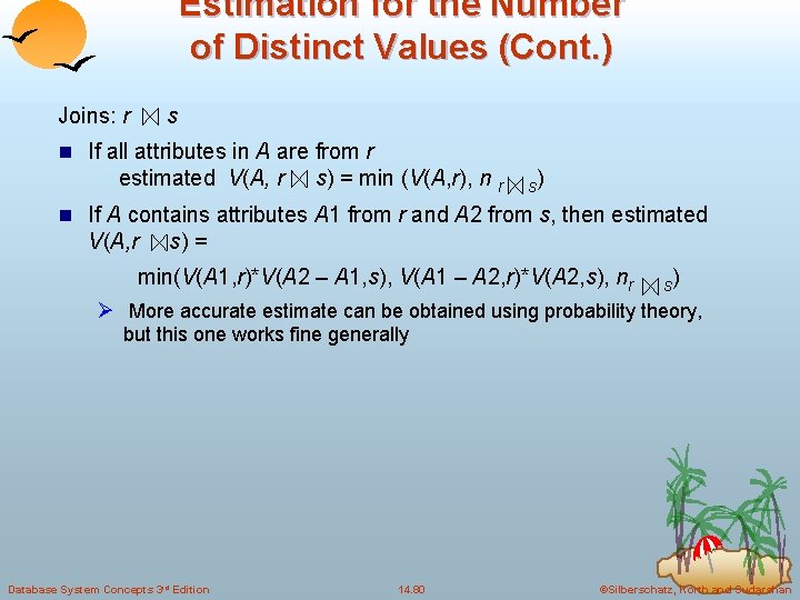
Estimation for the Number of Distinct Values (Cont. ) Joins: r s n If all attributes in A are from r estimated V(A, r s) = min (V(A, r), n r s) n If A contains attributes A 1 from r and A 2 from s, then estimated V(A, r s) = min(V(A 1, r)*V(A 2 – A 1, s), V(A 1 – A 2, r)*V(A 2, s), nr s) Ø More accurate estimate can be obtained using probability theory, but this one works fine generally Database System Concepts 3 rd Edition 14. 80 ©Silberschatz, Korth and Sudarshan

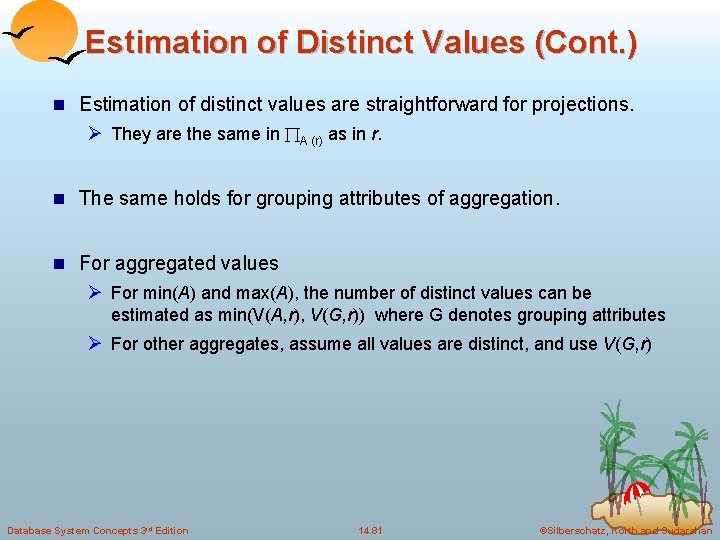
Estimation of Distinct Values (Cont. ) n Estimation of distinct values are straightforward for projections. Ø They are the same in A (r) as in r. n The same holds for grouping attributes of aggregation. n For aggregated values Ø For min(A) and max(A), the number of distinct values can be estimated as min(V(A, r), V(G, r)) where G denotes grouping attributes Ø For other aggregates, assume all values are distinct, and use V(G, r) Database System Concepts 3 rd Edition 14. 81 ©Silberschatz, Korth and Sudarshan