Chapter 14 Polynomial Interpolation Interpolation Extrapolation Interpolation data

Chapter 14 Polynomial Interpolation

Interpolation & Extrapolation • Interpolation: data to be found are within the range of observed data. • Extrapolation: data to be found are beyond the range of observation data. (not reliable*)

Interpolation Ø Used to estimate values between data points Ø Difference from regression Ø exactly goes through data points Ø therefore, no error at data points The most common method is the polynomial interpolation

Interpolation vs. Regression Same data points, different curve fitting

Polynomial Interpolation z Given n data points, fit a unique (n-1)th- order polynomial through them z Use polynomial interpolation to determine a’s z For consistency with MATLAB, use

Interpolating Polynomials First-order second-order third-order

Coefficients of an Interpolating Polynomial z Newton and Lagrange polynomials are well-suited for determining values between points (interpolation) z However, they do not provide a convenient polynomial of conventional form z Use n data points to determine n coefficients

Coefficients of an Interpolating Polynomial z Can be solved with any matrix method, but not efficient z There are more efficient methods to find p’s z The above equations are notoriously ill-conditioned, especially for large n z Limit yourself to lower-order polynomials

Polynomial Coefficients z Example – use last four points of Table 14. 1 Vandermonde Matrices

Vandermonde Matrices >> A=[250^3 250^2 250 1; 300^3 300^2 300 1; 400^3 400^2 400 1; 500^3 500^2 500 1] A = 15625000 62500 250 1 27000000 90000 300 1 64000000 160000 400 1 125000000 250000 500 1 >> b=[0. 675; 0. 616; 0. 525; 0. 457] b = 0. 6750 0. 6160 0. 5250 0. 4570 >> format long >> p = Ab p = -0. 0000260000 0. 00000427000000 -0. 0029370000 1. 183000000 >> cond(A) ans = 9. 306535523991324 e+009 ill-conditioned matrix

Newton Interpolation z. Use Newton’s “divided differences” of the functional values z. The lower order coefficients bi do not change when the order of interpolation is increased z. It is easy to add more data points and try a higher order polynomial

Newton Linear Interpolation Start with linear interpolation: f 1(x) = b 1 + b 2 (x x 1 ) Similar triangles

Newton Linear Interpolation z Newton linear interpolation formula z Example 1: interpolate e 2 using e 1 and e 5 z Example 2: Interpolate e 2 using e 1. 5 and e 2. 5

Newton Linear Interpolation

Accuracy of Interpolation Logarithmic function Linear estimates of ln(2) Small interval x provides a better estimate

Quadratic Interpolation z Quadratic interpolation – need three points z Use the parabola z This is the same as where

Quadratic Interpolation z To get the coefficients b’s z 1) Set x = x 1, get b 1 = f(x 1) z 2) Use b 1 and set x = x 2 to get b 2

Quadratic Interpolation z 3) Use b 1 and b 2, and set x = x 3 to get b 3 b 1 is a constant (0 th order) b 2 gives slope (finite difference) b 3 gives curvature (difference of finite differences)

Hand Calculation Example: interpolate e 2 using e 1, e 3, and e 5

Example – use different xi Example: interpolate e 2 using e 1, e 1. 5, and e 2. 5

Quadratic Interpolation

Quadratic Interpolation

Order of Interpolation Linear, quadratic and cubic estimates of ln(2) Logarithmic function Higher-order interpolation improves the estimate

Newton’s Interpolating Polynomials z General form for Newton’s interpolating polynomials z Bracketed functions are finite differences

Newton’s Divided Differences z First finite difference z Second finite difference z The difference of two finite differences

Newton’s Divided Differences The nth finite difference An iterative procedure 1. Evaluate all first-order finite differences; save f (x 1) for b 1 2. Evaluate second-order from firsts; save f [x 2, x 1] for b 2 3. Continue to nth-order, saving needed ones

Newton Interpolation z No need to solve a system of simultaneous equations z Spacing may be non-uniform and xi may be in arbitrary order

Newton Interpolation First Second Third Fourth Use the top element of each column (= bn) to evaluate the interpolated functional value f(x)

Percentage Relative Error Relative error decreases with increasing order of the interpolating polynomial The error is also sensitive to the position and sequence of the original data (x 1 , x 2 , x 3 , x 4 , …, xn)

Hand Calculations Newton Interpolation

Error Estimate z Error for Newton’s interpolating polynomial z Estimate from z. The leading term in the truncated polynomial z. Similar to the truncation error in a Taylor series

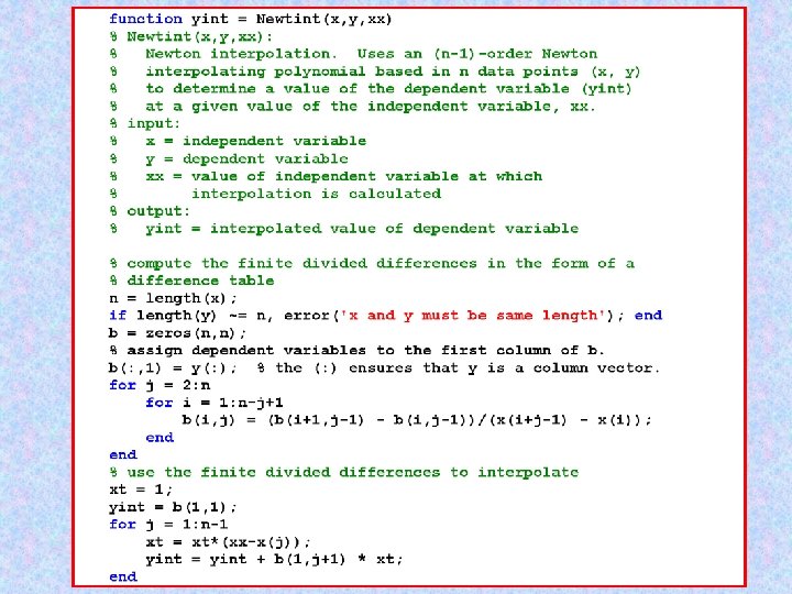
Modified M-File: yint may be evaluated at multiple points

Newton Interpolating Polynomial >> x = [0 x = 1 4 3 1. 5 2. 5] 0 1. 0000 4. 0000 3. 0000 1. 5000 2. 5000 >> y = exp(x) y = 1. 0000 2. 7183 54. 5982 20. 0855 4. 4817 12. 1825 Coefficients of >> xx = 0: 0. 1: 4; yy=exp(xx); Newton interpolating >> [b, yint] = Newtint 2(x, y, xx) b = polynomial 1. 0000 1. 7183 3. 8938 1. 5720 0. 3312 0. 0697 2. 7183 17. 2933 8. 6097 2. 0687 0. 5055 0 54. 5982 34. 5126 9. 6440 2. 8270 0 0 20. 0855 10. 4026 5. 4035 0 0 0 4. 4817 7. 7008 0 0 12. 1825 0 0 0 yint = Columns 1 through 8 1. 0000 1. 1355 1. 2670 1. 4000 1. 5394 1. 6893 1. 8536 2. 0356 Columns 9 through 16 2. 2384 2. 4651 2. 7183 3. 0008 3. 3153 3. 6649 4. 0525 4. 4817 Columns 17 through 24 4. 9561 5. 4801 6. 0584 6. 6964 7. 4003 8. 1770 9. 0343 9. 9809 Columns 25 through 32 11. 0266 12. 1825 13. 4606 14. 8744 16. 4387 18. 1698 20. 0855 22. 2054 Columns 33 through 40 24. 5506 27. 1441 30. 0107 33. 1774 36. 6729 40. 5284 44. 7770 49. 4543 Column 41 54. 5982 >> H = plot(x, y, 'mo', xx, yy, 'r', xx, yint, 'bx'); set(H, 'Line. Width', 3); Table

Newton Interpolation Polynomial f(x) = ex, Interpolation at [0 1 4 3 1. 5 2. 5]

Lagrange Interpolating Polynomials z Give the same result as the Newton’s polynomials, but different approach

Lagrange Interpolation z 1 st-order Lagrange polynomial z Second-order Lagrange polynomial z Third-order Lagrange polynomial

Linear Lagrange Interpolation Ø Both L 1(x) and L 2(x) are straight lines

Quadratic Lagrange Interpolation L 3(x)f(x 3) L 1(x)f(x 1) x 1 L 2(x)f(x 2) x 2 x 3

First-order Lagrange interpolation f(x) = ex Interpolation at [0 4]

Second-order Lagrange interpolation f(x) = ex, Interpolation at [0 1 4]

Third-order Lagrange interpolation f(x) = ex, Interpolation at [0 1 4 3]

Example: Lagrange Interpolation z Estimate f(x) = exp(x) at x = 2 using (x 0, x 1, x 2, x 3 ) = (0, 1, 4, 3) z second-order: (x 1, x 2, x 3 ) = (0, 1, 4) z third order: (x 1, x 2, x 3, x 4 ) = (0, 1, 4, 3)

Coefficients of Lagrange Polynomial Ø Save the coefficients of Lagrange polynomial Ø Evaluate the interpolated values at multiple locations

Evaluation of Interpolated Values

» x=[0 4] First-order x = 0 4 » y=exp(x) y = 1. 0000 54. 5982 » c=Lagrange_coef(x, y) c = -0. 2500 13. 6495 » t=2; p=Lagrange_eval(t, x, c) p = 27. 7991 » x=[0 1 4] Second-order x = 0 1 4 » y=exp(x) y = 1. 0000 2. 7183 54. 5982 » c=Lagrange_coef(x, y) c = 0. 2500 -0. 9061 4. 5498 » t=2; p=Lagrange_eval(t, x, c) p = 12. 2241 » x=[0 1 4 3] Third-order x = 0 1 4 3 » y=exp(x) y = 1. 0000 2. 7183 54. 5982 20. 0855 » c=Lagrange_coef(x, y) c = -0. 0833 0. 4530 4. 5498 -3. 3476 » t=2; p=Lagrange_eval(t, x, c) p = 5. 9362 Exact solution e 2 = 7. 389056

Lagrange Interpolation z. Very convenient for the same abscissas but different yi (e. g. , measurements always taken using the same independent variables xi) z. Lk(x) need to be computed only once z. However, it is less convenient when additional data may be added

Inverse Interpolation z Given x’s and f(x)’s – interpolation let us get new f(x) from new x z What about new x from new f(x)? z Example: f(x) = 1/x 1. Switch x and f(x) and do new interpolation. However, non-uniform spacing in [x vs. f(x)] often leads to oscillations in the resulting interpolating polynomial 2. Fit an nth-order polynomial to the original data [f(x) vs. x], then use root-finding techniques to find x.

Extrapolation should be avoided whenever possible

Dangers of Extrapolation Ø Use of a seventh-order polynomial to make a prediction of U. S. population in 2000 based on data from 1920 through 1990 Ø Reasonable to use interpolation, but not the extrapolation

Difficulties with Polynomial Interpolation Humped and Flat Data Runge’s function

Runge’s function » x 2=-1: 0. 2: 1 x 2 = Columns 1 through 7 -1. 0000 -0. 8000 -0. 6000 -0. 4000 Columns 8 through 11 0. 4000 0. 6000 0. 8000 1. 0000 » y 2=1. /(1+25*x 2. ^2) y 2 = Columns 1 through 7 0. 0385 0. 0588 0. 1000 0. 2000 Columns 8 through 11 0. 2000 0. 1000 0. 0588 0. 0385 » c=Lagrange_coef(x 2, y 2) c = Columns 1 through 7 0. 1035 -1. 5830 12. 1102 -64. 5875 Columns 8 through 11 -64. 5875 12. 1102 -1. 5830 0. 1035 » x=-1: 0. 02: 1; y=1. /(1+25*x. ^2); » t=x; p=Lagrange_eval(t, x 2, c); » H=plot(x, y, 'r', t, p, 'b-', x 2, y 2, 'mo'); » set(H, 'Line. Width', 2. 5) » print -djpeg 075 poly 5. jpg -0. 2000 0. 5000 1. 0000 0. 5000 282. 5702 -678. 1684 282. 5702

Oscillations

MATLAB Functions: polyfit and polyval >> x = linspace(-1, 1, 5); y = 1. /(1+25*x. ^2) >> xx = linspace(-1, 1); p = polyfit(x, y, 4) p = 3. 3156 0. 0000 -4. 2772 0. 0000 1. 0000 >> y 4 = polyval(p, xx); >> yr = 1. /(1+25*xx. ^2); >> H=plot(x, y, 'o', xx, y 4, xx, yr, '--') >> x=linspace(-1, 1, 11); y = 1. /(1+25*x. ^2) y = Columns 1 through 8 0. 0385 0. 0588 0. 1000 0. 2000 0. 5000 Columns 9 through 11 0. 1000 0. 0588 0. 0385 >> p = polyfit(x, y, 10) p = Columns 1 through 8 -220. 9417 0. 0000 494. 9095 -0. 0000 -381. 4338 Columns 9 through 11 -16. 8552 0. 0000 1. 0000 >> y 10 = polyval(p, xx); >> H = plot(x, y, 'o', xx, y 10, xx, yr, '--') >> set(H, 'Line. Width', 3, 'Marker. Size', 12) >> print -djpeg Fig 14_13. jpg 4 th-order polynomial 1. 0000 0. 5000 0. 2000 10 th-order polynomial 0. 0000 123. 3597 -0. 0000

Runge’s Function with polynomial fit 4 th-order 10 th-order

Noisy straight line function [x, y] = example x = [0. 00 0. 20 0. 80 1. 00 1. 20 1. 90 2. 00 2. 10 2. 95 3. 00]; y = [0. 01 0. 22 0. 76 1. 03 1. 18 1. 94 2. 01 2. 08 2. 90 2. 95]; » [x, y]=example x = Columns 1 through 7 0 0. 2000 0. 8000 1. 0000 1. 2000 Columns 8 through 10 2. 1000 2. 9500 3. 0000 y = Columns 1 through 7 0. 0100 0. 2200 0. 7600 1. 0300 1. 1800 Columns 8 through 10 2. 0800 2. 9000 2. 9500 » c=Lagrange_coef(x, y) c = Columns 1 through 7 -0. 0007 0. 0512 -2. 4384 8. 3366 -7. 7423 Columns 8 through 10 26. 4741 -1. 1493 0. 8958 » t=0: 0. 05: 3; p=Lagrange_eval(t, x, c); » H=plot(x, y, 'ro', t, p, 'b', x, x, 'm'); » set(H, 'Line. Width', 2. 5); print -djpeg 075 poly 4. jpg 1. 9000 2. 0000 1. 9400 2. 0100 37. 5192 -61. 2208

Noisy straight line

CVEN 302 -501 Homework No. 10 z Chapter 14 z Problem 14. 1(15) 14. 3(15), 14. 5 (20)(Hand Calculation) z Problem 14. 8 (20)(Hand Calculation and MATLAB program) z Chapter 15 z Problems 15. 2 (20), 15. 3 (20) (Hand Calculations) z Due on Wednesday 10/29/2008 at the beginning of the period