Chapter 14 Introduction to Inference 1202022 1 Statistical

Chapter 14 Introduction to Inference 1/20/2022 1

Statistical Inference Two forms of statistical inference: • Confidence intervals • Significance tests of hypotheses 1/20/2022 2

Population Mean μ We wish to infer population mean μ using sample mean “x-bar”. The following conditions prevail: 1. Data acquired by Simple Random Sample 2. Population distribution is Normal 3. The value of σ is known 4. The value of μ is NOT known 1/20/2022 3

Example • Statement of problem: Young people have a better chance of good jobs and wages if they are good with numbers. We want to know the average NAEP math score of a population. • Response variable ≡ NAEP math scores – – Range from 0 to 500 Have a Normal distribution Population standard deviation σ = 60 Population mean μ not known • A simple random sample of n = 840 individuals derives sample mean (“x-bar”) = 272 • We want to estimate population mean µ Reference: Rivera-Batiz, F. L. (1992). Quantitative literacy and the likelihood of employment among young adults. Journal of Human Resources, 27, 313 -328. 1/20/2022 4

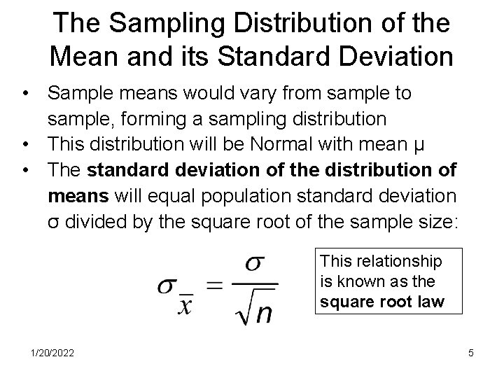
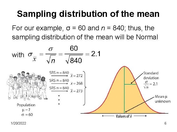
The Sampling Distribution of the Mean and its Standard Deviation • Sample means would vary from sample to sample, forming a sampling distribution • This distribution will be Normal with mean μ • The standard deviation of the distribution of means will equal population standard deviation σ divided by the square root of the sample size: This relationship is known as the square root law 1/20/2022 5

Sampling distribution of the mean For our example, σ = 60 and n = 840; thus, the sampling distribution of the mean will be Normal with 1/20/2022 6

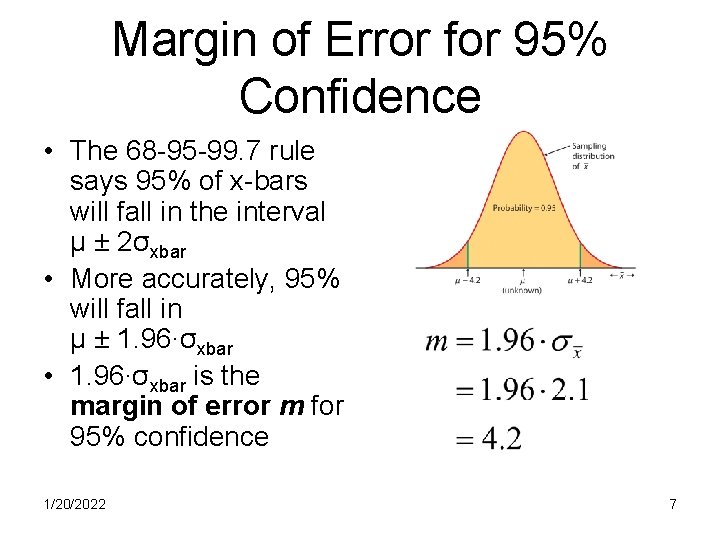
Margin of Error for 95% Confidence • The 68 -95 -99. 7 rule says 95% of x-bars will fall in the interval μ ± 2σxbar • More accurately, 95% will fall in μ ± 1. 96∙σxbar • 1. 96∙σxbar is the margin of error m for 95% confidence 1/20/2022 7

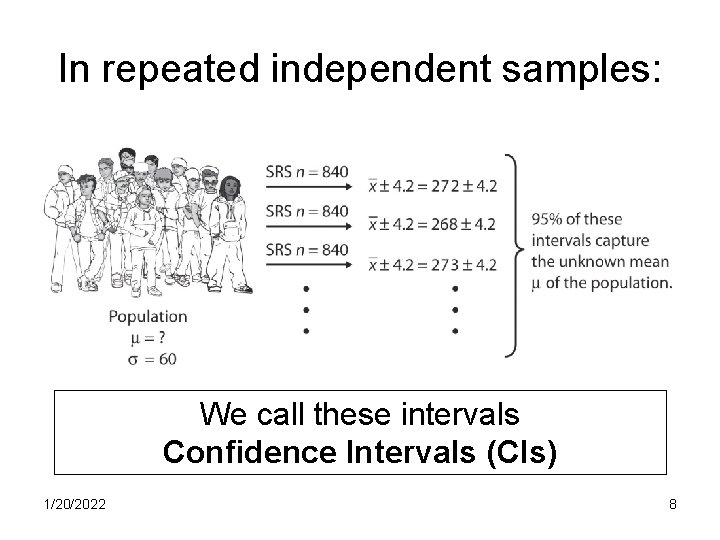
In repeated independent samples: We call these intervals Confidence Intervals (CIs) 1/20/2022 8

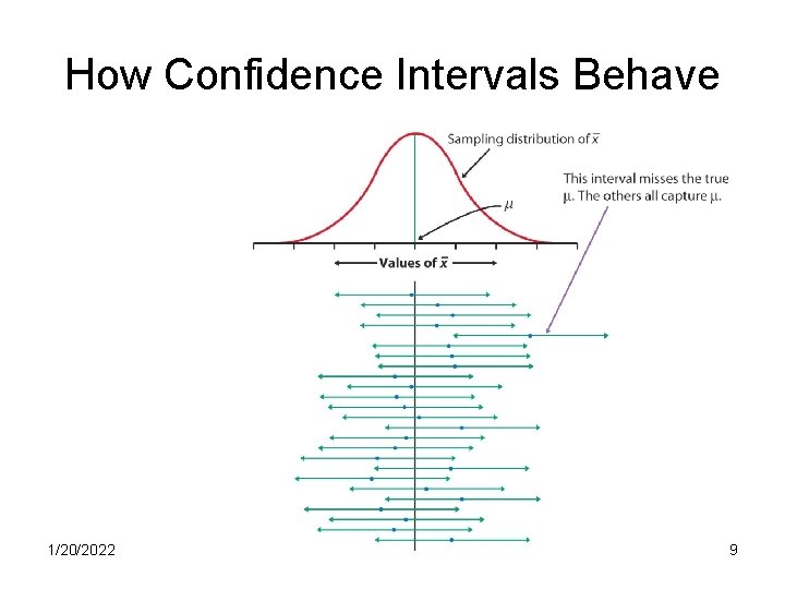
How Confidence Intervals Behave 1/20/2022 9

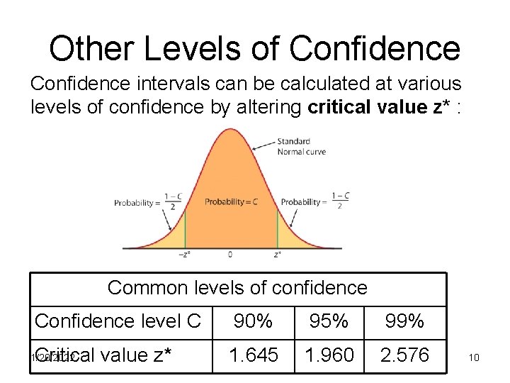
Other Levels of Confidence intervals can be calculated at various levels of confidence by altering critical value z* : Common levels of confidence Confidence level C 90% 95% 99% Critical value z* 1. 645 1. 960 2. 576 1/20/2022 10

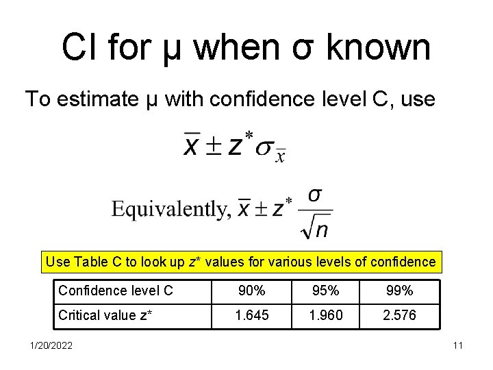
CI for μ when σ known To estimate μ with confidence level C, use Use Table C to look up z* values for various levels of confidence Confidence level C 90% 95% 99% Critical value z* 1. 645 1. 960 2. 576 1/20/2022 11

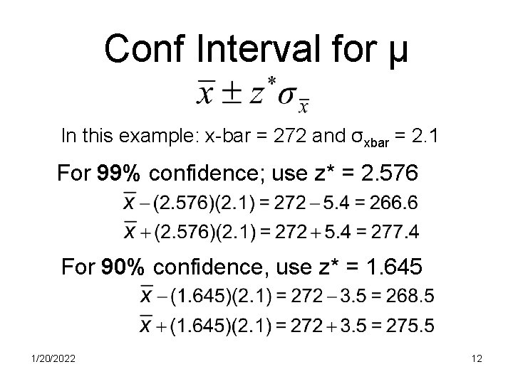
Conf Interval for μ In this example: x-bar = 272 and σxbar = 2. 1 For 99% confidence; use z* = 2. 576 For 90% confidence, use z* = 1. 645 1/20/2022 12

Tests of Significance • Recall: two forms of statistical inference – Confidence intervals – Hypothesis tests of significance • The objective of confidence intervals is to estimate a population parameter • The objective of a test of significance is to test a statistical hypothesis 1/20/2022 13

Tests of Significance: Reasoning • Like with confidence intervals, we ask what would happen if we repeated the sample or experiment many times • We assume the same conditions as before: (SRS, Normal population, population standard deviation σ known) • We recognize that sample means will vary from sample to sample • The text explains the reasoning behind tests of significance on pp. 369 – 376 20 January 2022 Basics of Significance Testing 14

Tests of Statistical Significance: Procedure A. The claim is stated as a null hypothesis H 0 and alternative hypotheses Ha B. Calculate a test statistic C. The test statistic is converted to a probability statement called a P-value D. The P-value is interpreted in terms of the weight of evidence against H 0 20 January 2022 Basics of Significance Testing 15

Example • Example: We want to test whether data in a sample provides reliable evidence that a population has gained weight. • Based on prior research, we know that weight gain in the population is Normal with σ = 1 lb • We select n = 10 individuals • The sample mean weight gain x-bar = 1. 02 lbs. • Is this level of evidence strong enough to conclude a population weight gain? 1/20/2022 16

The Null Hypothesis • The null hypothesis H 0 is a statement of “no difference” in the form: H 0: μ = μ 0 where μ 0 represents the value of the population if the null hypothesis is true • In our example, μ 0 = 0 and the null hypothesis is H 0: μ = 0 • Does the sample mean of 1. 02 based on n = 10 provide strong evidence that the null hypothesis is untrue? 1/20/2022 9: Basics of Hypothesis Testing 17

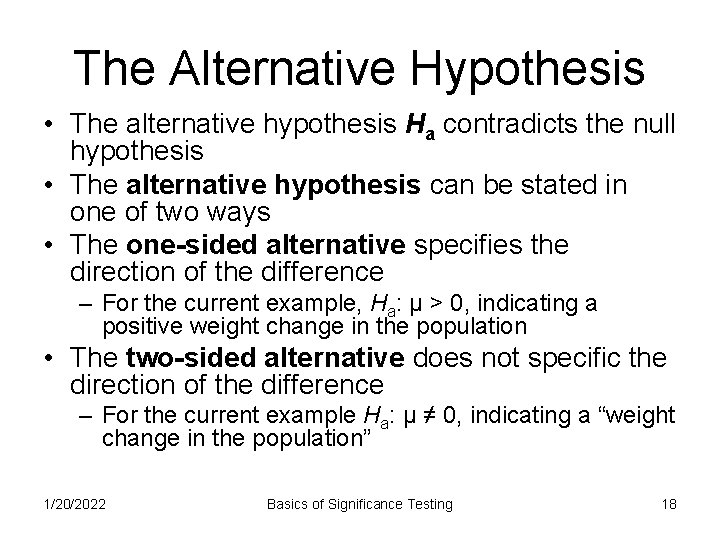
The Alternative Hypothesis • The alternative hypothesis Ha contradicts the null hypothesis • The alternative hypothesis can be stated in one of two ways • The one-sided alternative specifies the direction of the difference – For the current example, Ha: μ > 0, indicating a positive weight change in the population • The two-sided alternative does not specific the direction of the difference – For the current example Ha: μ ≠ 0, indicating a “weight change in the population” 1/20/2022 Basics of Significance Testing 18

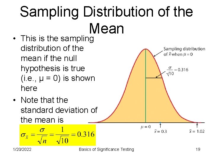
Sampling Distribution of the Mean • This is the sampling distribution of the mean if the null hypothesis is true (i. e. , μ = 0) is shown here • Note that the standard deviation of the mean is 1/20/2022 Basics of Significance Testing 19

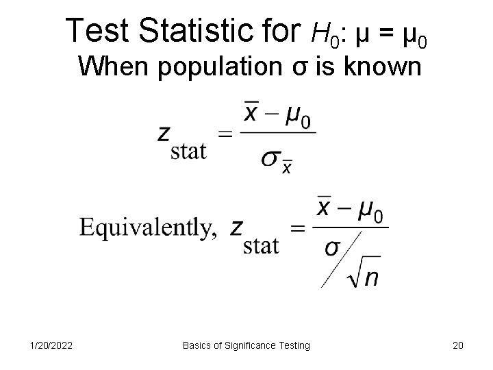
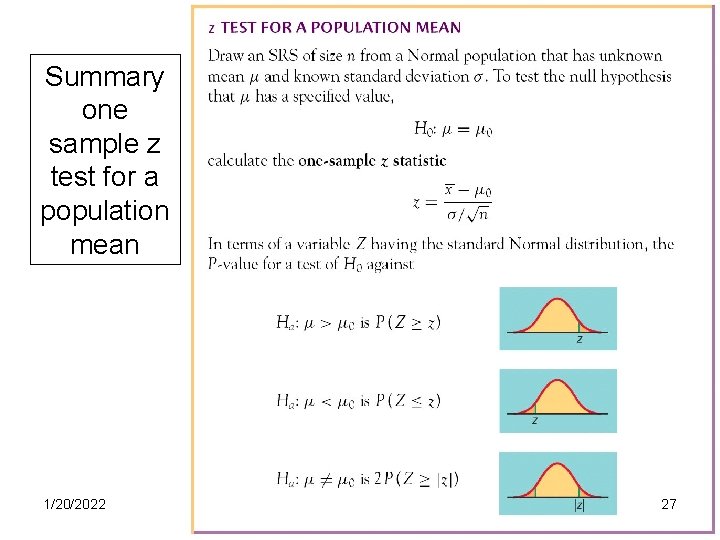
Test Statistic for H 0: μ = μ 0 When population σ is known 1/20/2022 Basics of Significance Testing 20

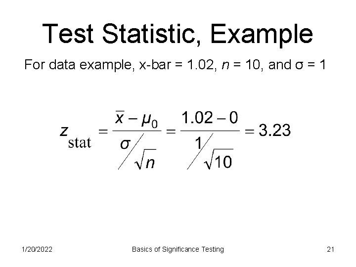
Test Statistic, Example For data example, x-bar = 1. 02, n = 10, and σ = 1 1/20/2022 Basics of Significance Testing 21

P-Value from z table Convert z statistics to a P-value: • For Ha: μ > μ 0 P-value = Pr(Z > zstat) = right-tail beyond zstat • For Ha: μ < μ 0 P-value = Pr(Z < zstat) = left tail beyond zstat • For Ha: μ ¹ μ 0 P-value = 2 × one-tailed P-value 1/20/2022 Basics of Significance Testing 22

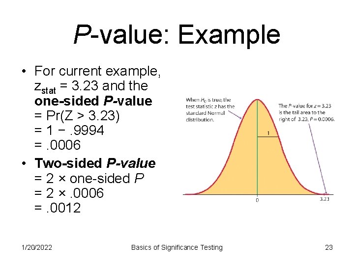
P-value: Example • For current example, zstat = 3. 23 and the one-sided P-value = Pr(Z > 3. 23) = 1 −. 9994 =. 0006 • Two-sided P-value = 2 × one-sided P = 2 ×. 0006 =. 0012 1/20/2022 Basics of Significance Testing 23

P-value: Interpretation • P-value (definition) ≡ the probability the sample mean would take a value as extreme or more extreme than observed test statistic when H 0 is true • P-value (interpretation) Smaller-and-smaller P-values → stronger-and-stronger evidence against H 0 • P-value (conventions). 10 < P < 1. 0 evidence against H 0 is not significant. 05 < P ≤. 10 evidence against H 0 is marginally signif. . 01 < P ≤. 05 evidence against H 0 is significant 0 < P ≤. 01 evidence against H 0 is highly significant 1/20/2022 Basics of Significance Testing 24

P-value: Example • Let us interpret the current two-sided P-value of. 0012 • This provides strong evidence against H 0 • Thus, we reject H 0 and say there is highly significant evidence of a weight gain in the population 1/20/2022 Basics of Significance Testing 25

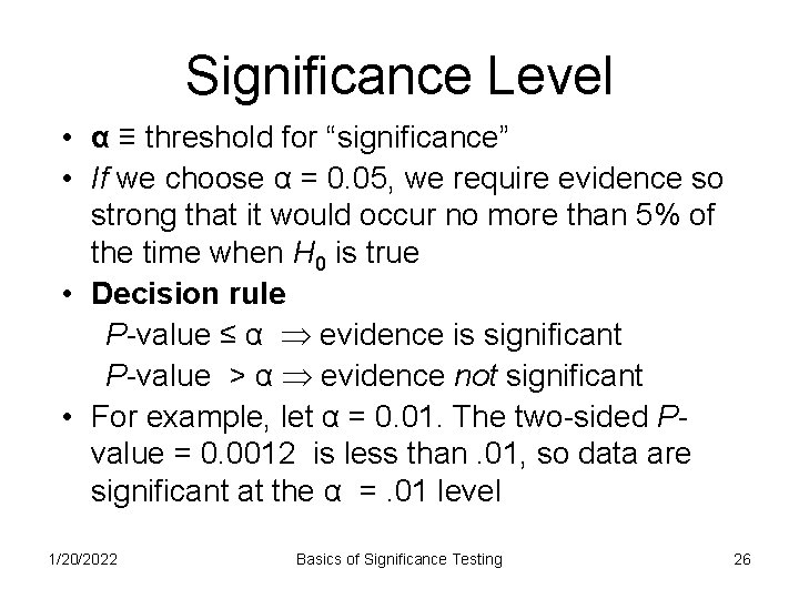
Significance Level • α ≡ threshold for “significance” • If we choose α = 0. 05, we require evidence so strong that it would occur no more than 5% of the time when H 0 is true • Decision rule P-value ≤ α evidence is significant P-value > α evidence not significant • For example, let α = 0. 01. The two-sided Pvalue = 0. 0012 is less than. 01, so data are significant at the α =. 01 level 1/20/2022 Basics of Significance Testing 26

Summary one sample z test for a population mean 1/20/2022 Basics of Significance Testing 27