CHAPTER 14 Design Of Experiments With Several Factors

CHAPTER 14 Design Of Experiments With Several Factors

LEARNING OBJECTIVES • Design and conduct engineering experiments involving several factors • Analyze and interpret main effects and interactions • How the ANOVA is used to analyze the data • Use the two-level series of factorial designs • Design and conduct two-level fractional factorial designs

Factorial Experimental Design • Performed in all engineering disciplines – Learn about how systems and processes work • Focus on experiments that include two or more factors • Experimental trials are performed at all combinations of factor levels • Single-factor experiments can be extended to the factorial experiments • ANOVA as the primary tools

FACTORIAL EXPERIMENTS • Factorial experimental design should be used • Mean that in each complete trial all possible combinations of the levels • Two factors A and B with a levels of factor A and b levels of factor B

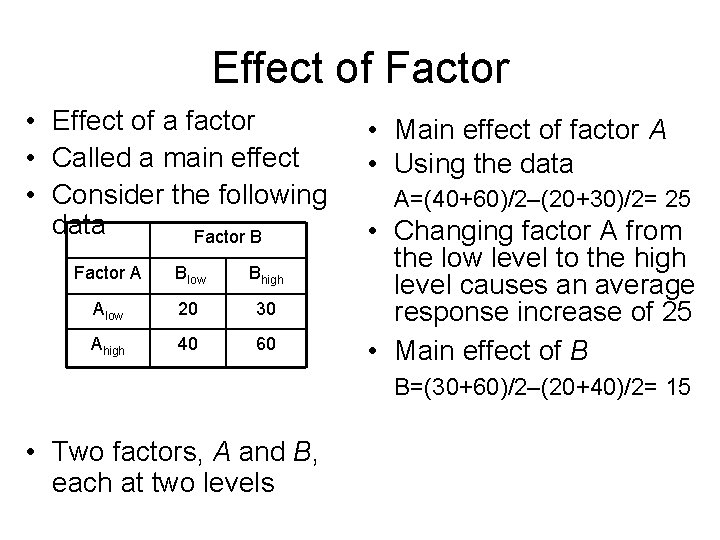
Effect of Factor • Effect of a factor • Called a main effect • Consider the following data Factor B Factor A Blow Bhigh Alow 20 30 Ahigh 40 60 • Main effect of factor A • Using the data A=(40+60)/2–(20+30)/2= 25 • Changing factor A from the low level to the high level causes an average response increase of 25 • Main effect of B B=(30+60)/2–(20+40)/2= 15 • Two factors, A and B, each at two levels

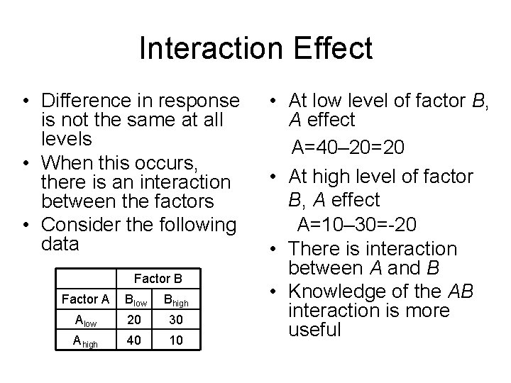
Interaction Effect • Difference in response is not the same at all levels • When this occurs, there is an interaction between the factors • Consider the following data Factor B Factor A Blow Bhigh Alow 20 30 Ahigh 40 10 • At low level of factor B, A effect A=40– 20=20 • At high level of factor B, A effect A=10– 30=-20 • There is interaction between A and B • Knowledge of the AB interaction is more useful

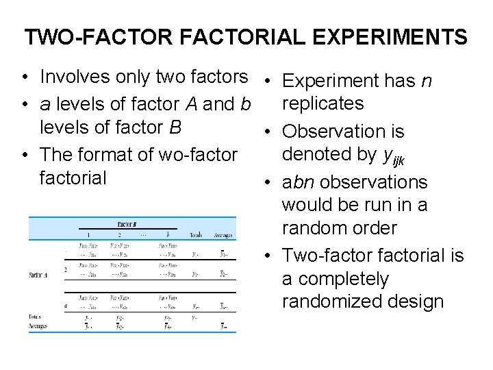
TWO-FACTORIAL EXPERIMENTS • Involves only two factors • Experiment has n replicates • a levels of factor A and b levels of factor B • Observation is denoted by yijk • The format of wo-factorial • abn observations would be run in a random order • Two-factorial is a completely randomized design

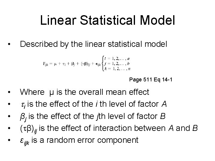
Linear Statistical Model • Described by the linear statistical model Page 511 Eq 14 -1 • • • Where µ is the overall mean effect i is the effect of the i th level of factor A βj is the effect of the jth level of factor B ( β)ij is the effect of interaction between A and B εijk is a random error component

Testing The Hypotheses • Interested in testing the hypotheses • Analysis of variance (ANOVA) will be used to test these hypotheses • Test procedure is sometimes called the two-way analysis of variance • A and B are fixed factors • Chosen by the experimenter • Test hypotheses about the main factor effects of A and B and the AB • Need some symbols

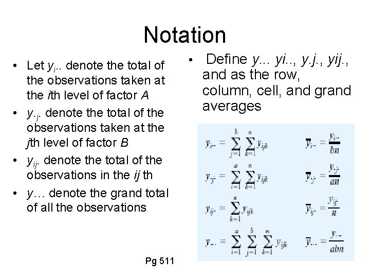
Notation • Let yi. . denote the total of the observations taken at the ith level of factor A • y. j. denote the total of the observations taken at the jth level of factor B • yij. denote the total of the observations in the ij th • y… denote the grand total of all the observations Pg 511 • Define y. . . yi. . , y. j. , yij. , and as the row, column, cell, and grand averages

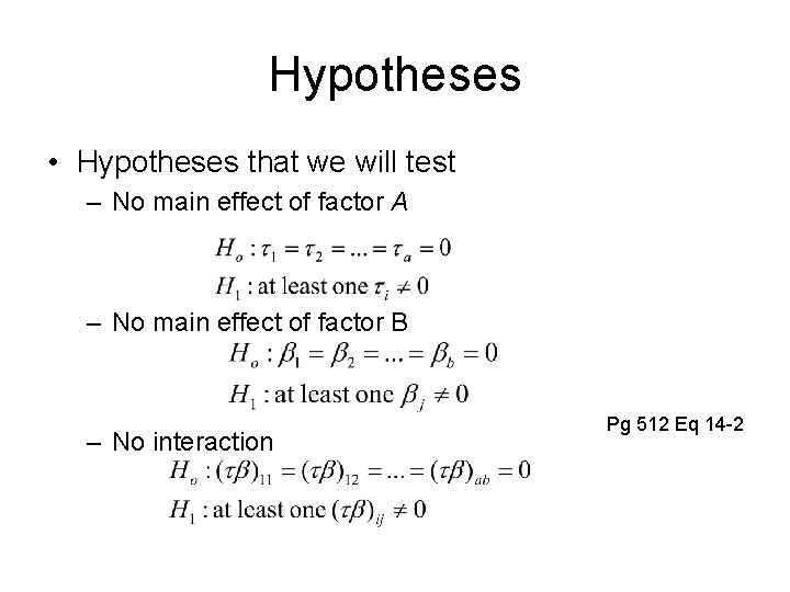
Hypotheses • Hypotheses that we will test – No main effect of factor A – No main effect of factor B – No interaction Pg 512 Eq 14 -2

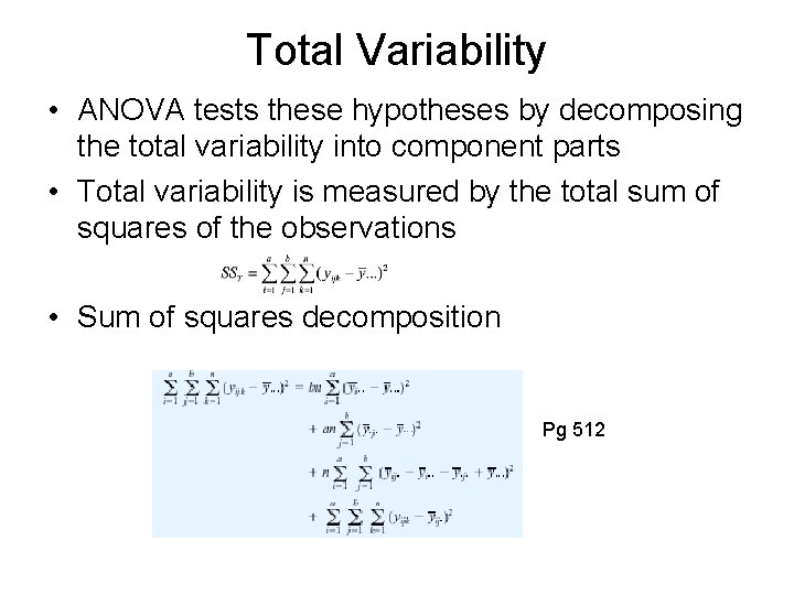
Total Variability • ANOVA tests these hypotheses by decomposing the total variability into component parts • Total variability is measured by the total sum of squares of the observations • Sum of squares decomposition Pg 512

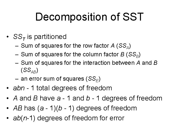
Decomposition of SST • SST is partitioned – Sum of squares for the row factor A (SSA) – Sum of squares for the column factor B (SSB) – Sum of squares for the interaction between A and B (SSAB) – an error sum of squares (SSE) • • abn - 1 total degrees of freedom A and B have a - 1 and b - 1 degrees of freedom AB has (a - 1)(b - 1) degrees of freedom ab(n-1) degrees of freedom for error

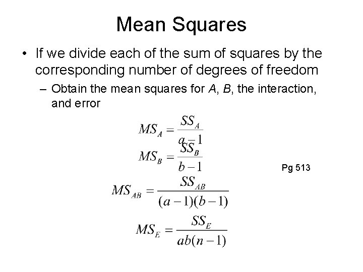
Mean Squares • If we divide each of the sum of squares by the corresponding number of degrees of freedom – Obtain the mean squares for A, B, the interaction, and error Pg 513

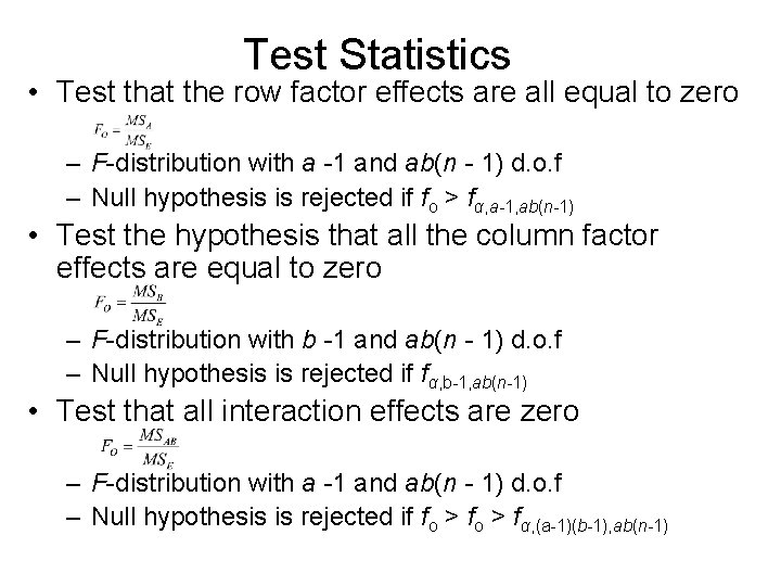
Test Statistics • Test that the row factor effects are all equal to zero – F-distribution with a -1 and ab(n - 1) d. o. f – Null hypothesis is rejected if fo > fα, a-1, ab(n-1) • Test the hypothesis that all the column factor effects are equal to zero – F-distribution with b -1 and ab(n - 1) d. o. f – Null hypothesis is rejected if fα, b-1, ab(n-1) • Test that all interaction effects are zero – F-distribution with a -1 and ab(n - 1) d. o. f – Null hypothesis is rejected if fo > fα, (a-1)(b-1), ab(n-1)

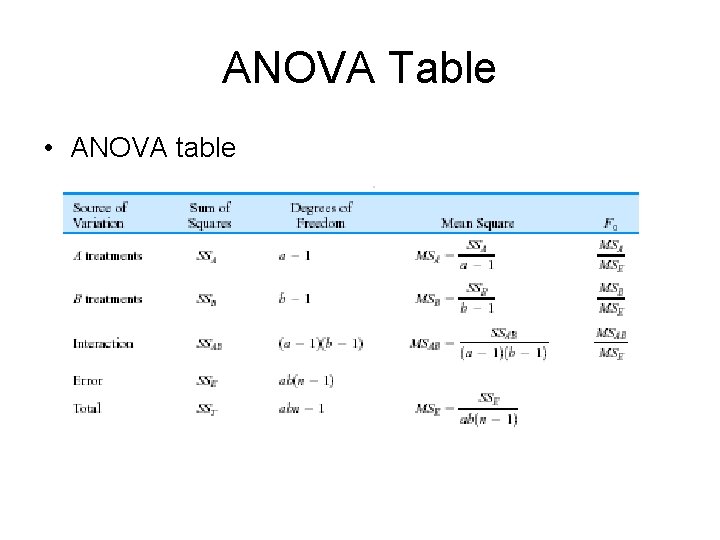
ANOVA Table • ANOVA table

Interaction or Main Effects? • Conduct the test for interaction first • Interpretation of the tests on the main effects • When interaction is significant – Main effects of the factors may not have much practical interpretative value

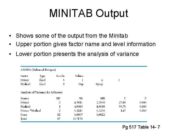
MINITAB Output • Shows some of the output from the Minitab • Upper portion gives factor name and level information • Lower portion presents the analysis of variance Pg 517 Table 14 - 7

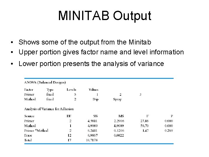
MINITAB Output • Shows some of the output from the Minitab • Upper portion gives factor name and level information • Lower portion presents the analysis of variance

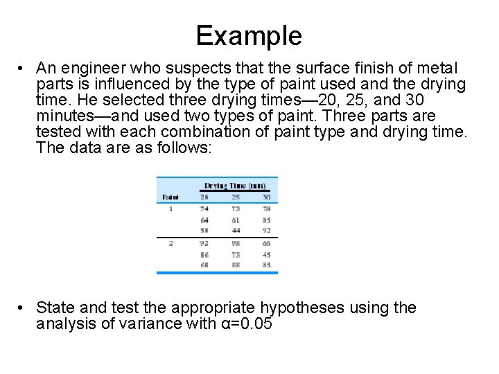
Example • An engineer who suspects that the surface finish of metal parts is influenced by the type of paint used and the drying time. He selected three drying times— 20, 25, and 30 minutes—and used two types of paint. Three parts are tested with each combination of paint type and drying time. The data are as follows: • State and test the appropriate hypotheses using the analysis of variance with α=0. 05

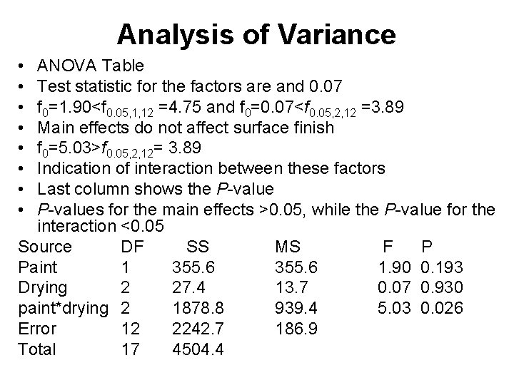
Analysis of Variance • • ANOVA Table Test statistic for the factors are and 0. 07 f 0=1. 90<f 0. 05, 1, 12 =4. 75 and f 0=0. 07<f 0. 05, 2, 12 =3. 89 Main effects do not affect surface finish f 0=5. 03>f 0. 05, 2, 12= 3. 89 Indication of interaction between these factors Last column shows the P-values for the main effects >0. 05, while the P-value for the interaction <0. 05 Source DF SS MS F P Paint 1 355. 6 1. 90 0. 193 Drying 2 27. 4 13. 7 0. 07 0. 930 paint*drying 2 1878. 8 939. 4 5. 03 0. 026 Error 12 2242. 7 186. 9 Total 17 4504. 4

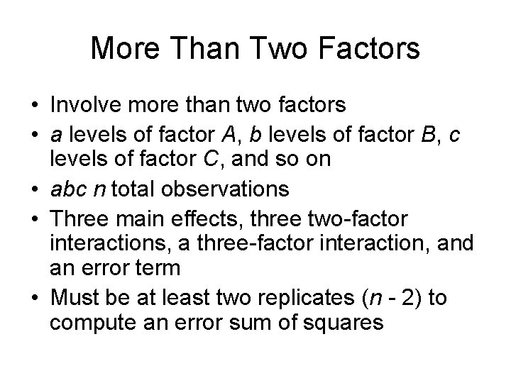
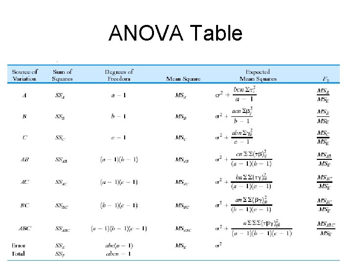
More Than Two Factors • Involve more than two factors • a levels of factor A, b levels of factor B, c levels of factor C, and so on • abc n total observations • Three main effects, three two-factor interactions, a three-factor interaction, and an error term • Must be at least two replicates (n - 2) to compute an error sum of squares

ANOVA Table

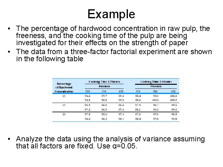
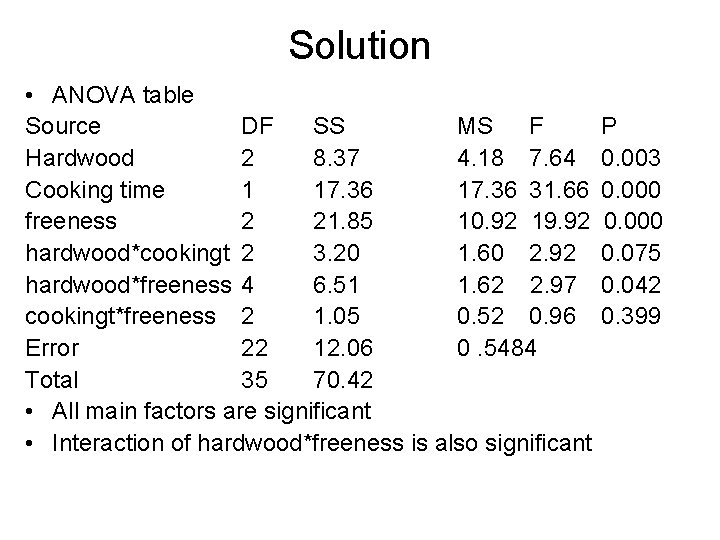
Example • The percentage of hardwood concentration in raw pulp, the freeness, and the cooking time of the pulp are being investigated for their effects on the strength of paper • The data from a three-factorial experiment are shown in the following table • Analyze the data using the analysis of variance assuming that all factors are fixed. Use α=0. 05.

Solution • ANOVA table Source DF SS MS F Hardwood 2 8. 37 4. 18 7. 64 Cooking time 1 17. 36 31. 66 freeness 2 21. 85 10. 92 19. 92 hardwood*cookingt 2 3. 20 1. 60 2. 92 hardwood*freeness 4 6. 51 1. 62 2. 97 cookingt*freeness 2 1. 05 0. 52 0. 96 Error 22 12. 06 0. 5484 Total 35 70. 42 • All main factors are significant • Interaction of hardwood*freeness is also significant P 0. 003 0. 000 0. 075 0. 042 0. 399

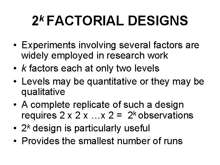
2 k FACTORIAL DESIGNS • Experiments involving several factors are widely employed in research work • k factors each at only two levels • Levels may be quantitative or they may be qualitative • A complete replicate of such a design requires 2 x …x 2 = 2 k observations • 2 k design is particularly useful • Provides the smallest number of runs

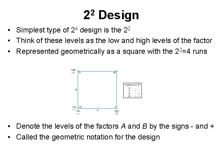
22 Design • Simplest type of 2 k design is the 22 • Think of these levels as the low and high levels of the factor • Represented geometrically as a square with the 22=4 runs • Denote the levels of the factors A and B by the signs - and + • Called the geometric notation for the design

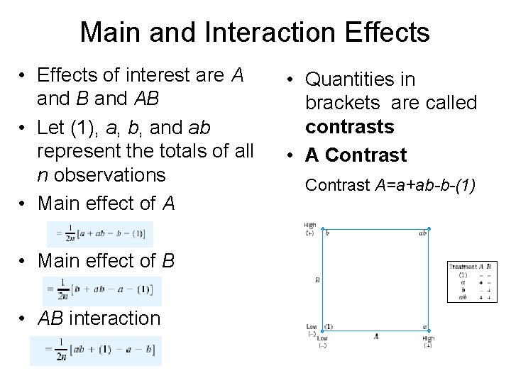
Main and Interaction Effects • Effects of interest are A and B and AB • Let (1), a, b, and ab represent the totals of all n observations • Main effect of A • Main effect of B • AB interaction • Quantities in brackets are called contrasts • A Contrast A=a+ab-b-(1)

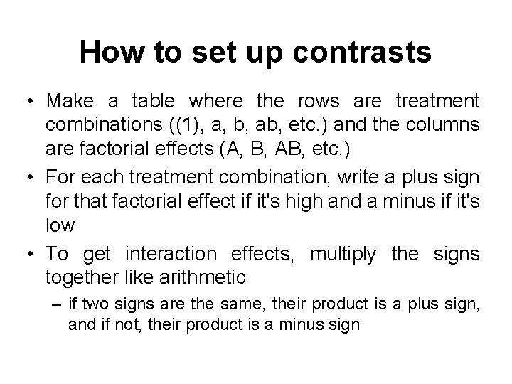
How to set up contrasts • Make a table where the rows are treatment combinations ((1), a, b, ab, etc. ) and the columns are factorial effects (A, B, AB, etc. ) • For each treatment combination, write a plus sign for that factorial effect if it's high and a minus if it's low • To get interaction effects, multiply the signs together like arithmetic – if two signs are the same, their product is a plus sign, and if not, their product is a minus sign

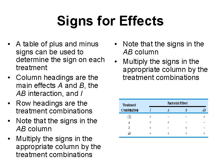
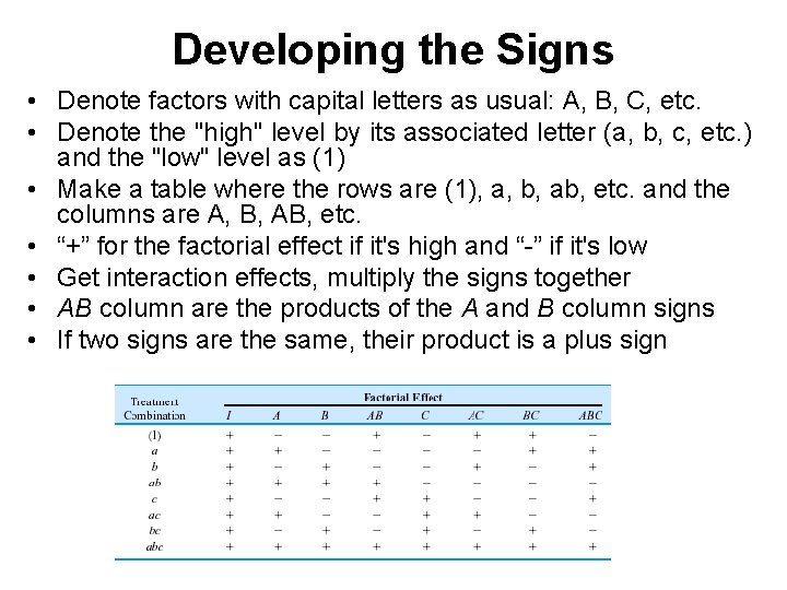
Signs for Effects • A table of plus and minus signs can be used to determine the sign on each treatment • Column headings are the main effects A and B, the AB interaction, and I • Row headings are the treatment combinations • Note that the signs in the AB column • Multiply the signs in the appropriate column by the treatment combinations

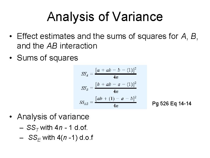
Analysis of Variance • Effect estimates and the sums of squares for A, B, and the AB interaction • Sums of squares Pg 526 Eq 14 -14 • Analysis of variance – SST with 4 n - 1 d. of. – SSE with 4(n -1) d. o. f

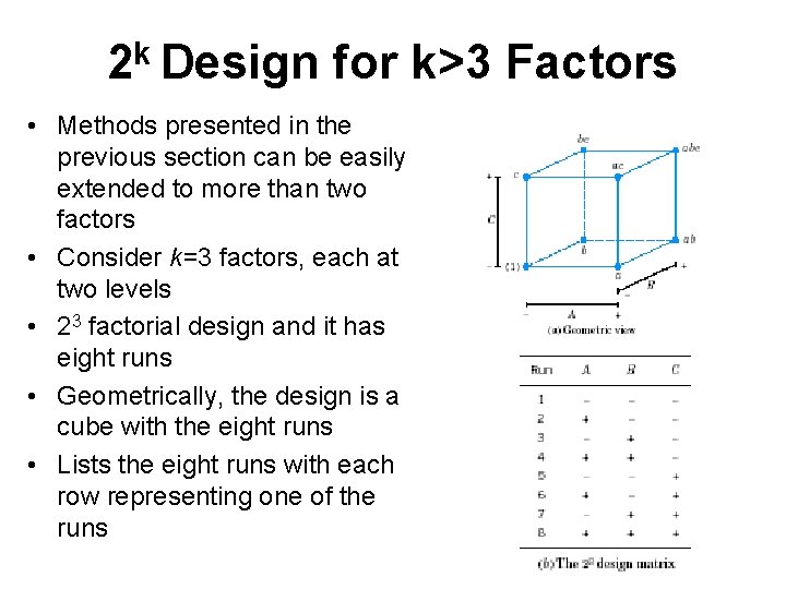
k 2 Design for k>3 Factors • Methods presented in the previous section can be easily extended to more than two factors • Consider k=3 factors, each at two levels • 23 factorial design and it has eight runs • Geometrically, the design is a cube with the eight runs • Lists the eight runs with each row representing one of the runs

Developing the Signs • Denote factors with capital letters as usual: A, B, C, etc. • Denote the "high" level by its associated letter (a, b, c, etc. ) and the "low" level as (1) • Make a table where the rows are (1), a, b, ab, etc. and the columns are A, B, AB, etc. • “+” for the factorial effect if it's high and “-” if it's low • Get interaction effects, multiply the signs together • AB column are the products of the A and B column signs • If two signs are the same, their product is a plus sign

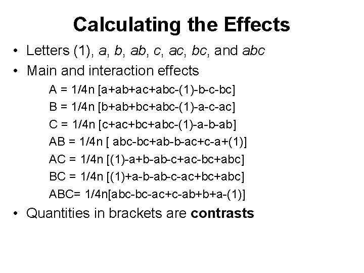
Calculating the Effects • Letters (1), a, b, ab, c, ac, bc, and abc • Main and interaction effects A = 1/4 n [a+ab+ac+abc-(1)-b-c-bc] B = 1/4 n [b+ab+bc+abc-(1)-a-c-ac] C = 1/4 n [c+ac+bc+abc-(1)-a-b-ab] AB = 1/4 n [ abc-bc+ab-b-ac+c-a+(1)] AC = 1/4 n [(1)-a+b-ab-c+ac-bc+abc] BC = 1/4 n [(1)+a-b-ab-c-ac+bc+abc] ABC= 1/4 n[abc-bc-ac+c-ab+b+a-(1)] • Quantities in brackets are contrasts

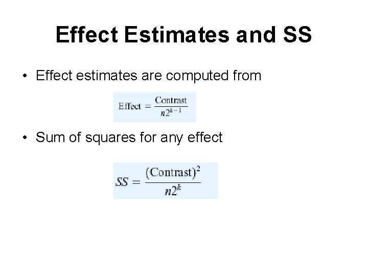
Effect Estimates and SS • Effect estimates are computed from • Sum of squares for any effect

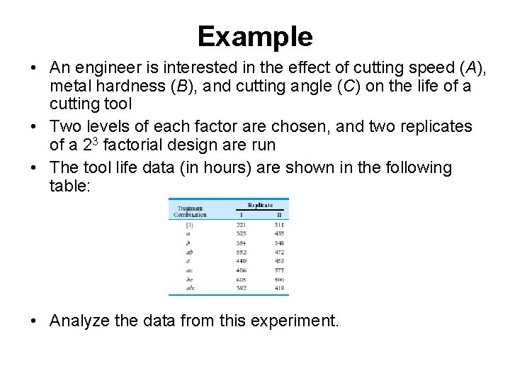
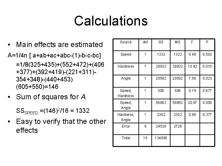
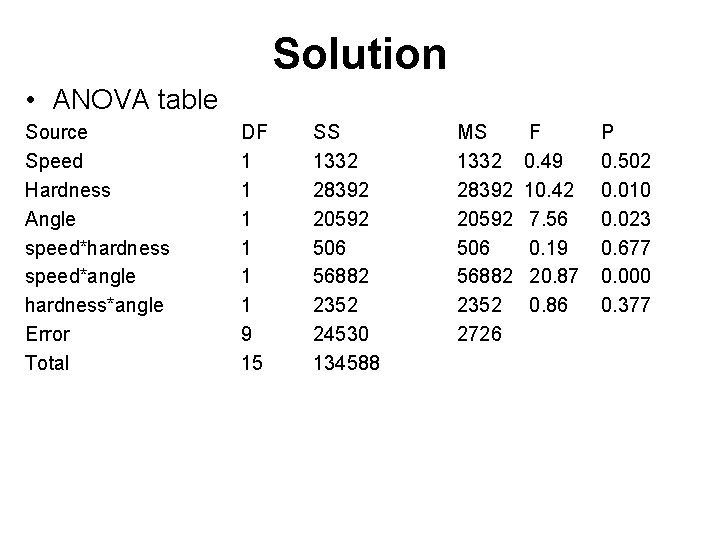
Example • An engineer is interested in the effect of cutting speed (A), metal hardness (B), and cutting angle (C) on the life of a cutting tool • Two levels of each factor are chosen, and two replicates of a 23 factorial design are run • The tool life data (in hours) are shown in the following table: • Analyze the data from this experiment.

Calculations • Main effects are estimated Source dof SS MS F P A=1/4 n [ a+ab+ac+abc-(1)-b-c-bc] =1/8(325+435)+(552+472)+(406 +377)+(392+419)-(221+311)354+348)-(440+453) (605+550)=146 Speed 1 1332 1322 0. 49 0. 502 Hardness 1 28932 10. 42 0. 010 Angle 1 20592 7. 56 0. 023 Speed, Hardness 1 506 0. 19 0. 677 Speed, Angle 1 56882 20. 87 0. 000 Hardness, Angle 1 2352 0. 86 0. 377 Error 9 24530 2726 Total 15 134588 • Sum of squares for A SSSPEED =(146)2/16 = 1332 • Easy to verify that the other effects

Solution • ANOVA table Source Speed Hardness Angle speed*hardness speed*angle hardness*angle Error Total DF 1 1 1 9 15 SS 1332 28392 20592 506 56882 2352 24530 134588 MS 1332 28392 20592 506 56882 2352 2726 F 0. 49 10. 42 7. 56 0. 19 20. 87 0. 86 P 0. 502 0. 010 0. 023 0. 677 0. 000 0. 377

Next Agenda • Methods and applications of nonparametric statistics