Chapter 13 Time Series Analysis and Index Numbers

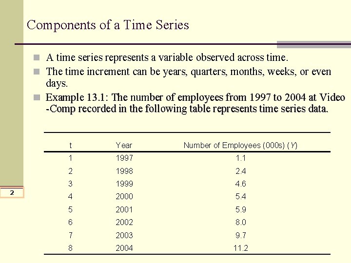
Components of a Time Series n A time series represents a variable observed across time. n The time increment can be years, quarters, months, weeks, or even days. n Example 13. 1: The number of employees from 1997 to 2004 at Video -Comp recorded in the following table represents time series data. 2 t Year Number of Employees (000 s) (Y) 1 1997 1. 1 2 1998 2. 4 3 1999 4. 6 4 2000 5. 4 5 2001 5. 9 6 2002 8. 0 7 2003 9. 7 8 2004 11. 2

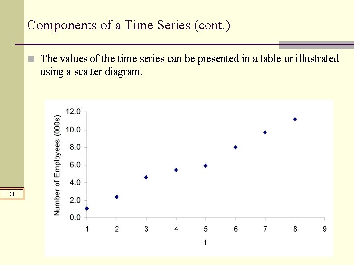
Components of a Time Series (cont. ) n The values of the time series can be presented in a table or illustrated using a scatter diagram. 3

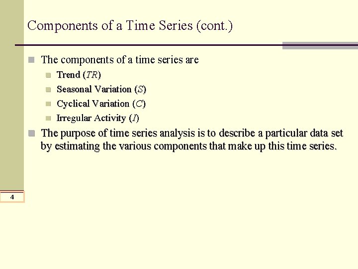
Components of a Time Series (cont. ) n The components of a time series are n Trend (TR) n Seasonal Variation (S) n Cyclical Variation (C) n Irregular Activity (I) n The purpose of time series analysis is to describe a particular data set by estimating the various components that make up this time series. 4

Trend (TR) n Steady increase or decrease in the time series. n Reflects any long-term growth or decline in the observations. n A trend may be due to inflation, increases in the population, increases in personal income, market growth or decline, or change in technology. n Usually follows a straight line (linear trend), but can also be curvilinear (quadratic trend). 5

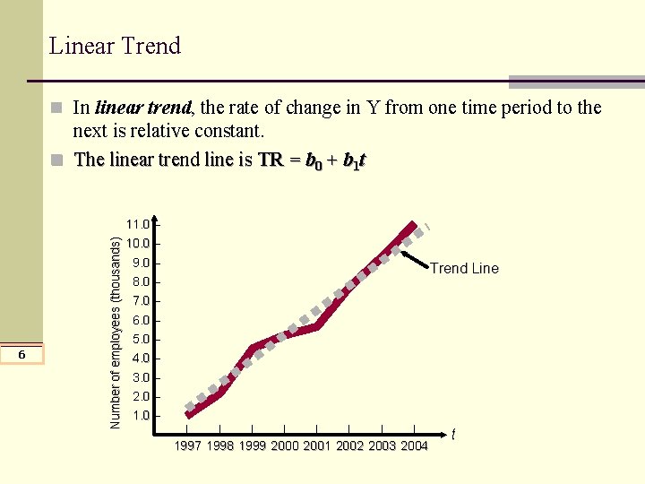
Linear Trend n In linear trend, the rate of change in Y from one time period to the 6 Number of employees (thousands) next is relative constant. n The linear trend line is TR = b 0 + b 1 t 11. 0 – 10. 0 – 9. 0 – 8. 0 – Trend Line 7. 0 – 6. 0 – 5. 0 – 4. 0 – 3. 0 – 2. 0 – 1. 0 – | | | | 1997 1998 1999 2000 2001 2002 2003 2004 t

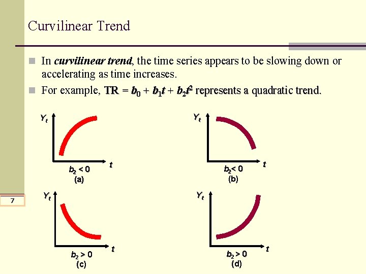
Curvilinear Trend n In curvilinear trend, the time series appears to be slowing down or accelerating as time increases. n For example, TR = b 0 + b 1 t + b 2 t 2 represents a quadratic trend. Yt Yt b 2 < 0 (a) 7 t b 2< 0 (b) t Yt Yt b 2 > 0 (c) t b 2 > 0 (d) t

Seasonality (S) n Seasonal variation refers to periodic increases or decreases that occur n n within a calendar year in a time series. The key is that these movements in the time series follow the same pattern each year. For example, sales are always high in December. Monthly or quarterly data. Annual data can not be used to examine seasonality. Two types of seasonal variation n 8 n Additive seasonality Multiplicative seasonality (usually the case)

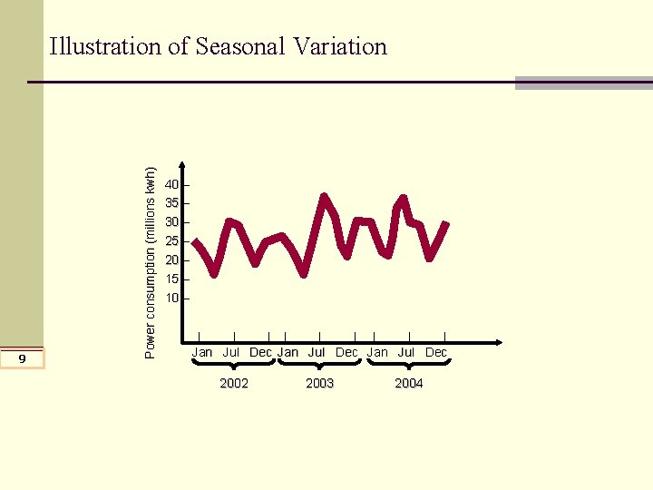
9 Power consumption (millions kwh) Illustration of Seasonal Variation 40 – 35 – 30 – 25 – 20 – 15 – 10 – | | | | | Jan Jul Dec 2002 2003 2004

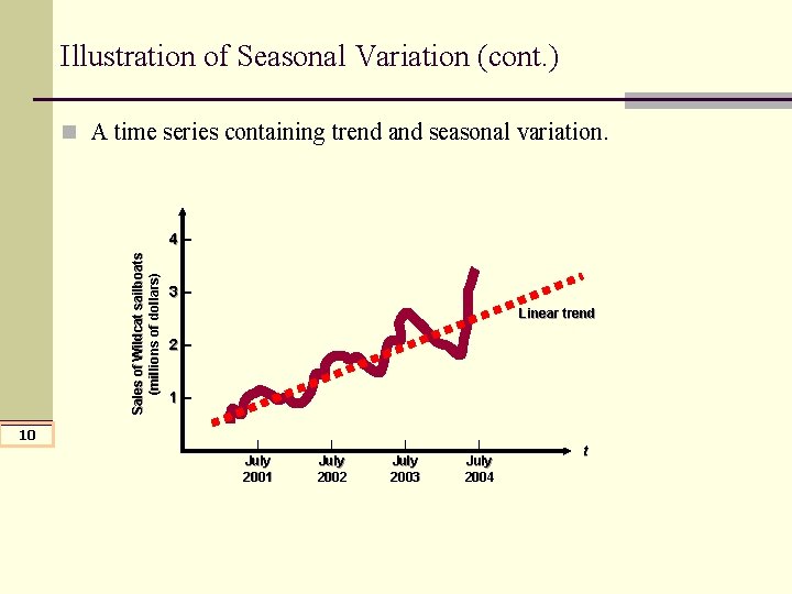
Illustration of Seasonal Variation (cont. ) n A time series containing trend and seasonal variation. Sales of Wildcat sailboats (millions of dollars) 4– 10 3– Linear trend 2– 1– | July 2001 | July 2002 | July 2003 | July 2004 t

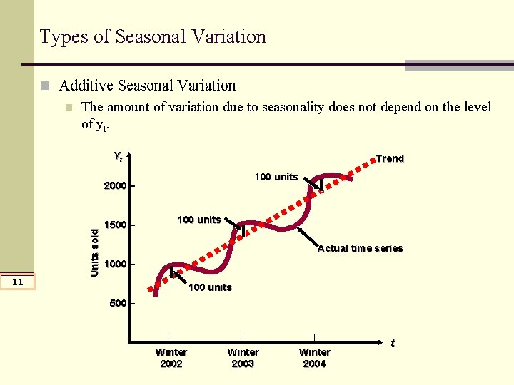
Types of Seasonal Variation n Additive Seasonal Variation n The amount of variation due to seasonality does not depend on the level of yt. Yt Trend 100 units 11 Units sold 2000 – 1500 – 100 units Actual time series 1000 – 100 units 500 – | Winter 2002 | Winter 2003 | Winter 2004 t

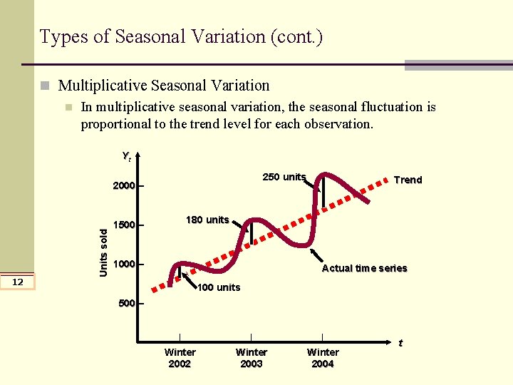
Types of Seasonal Variation (cont. ) n Multiplicative Seasonal Variation n In multiplicative seasonal variation, the seasonal fluctuation is proportional to the trend level for each observation. Yt 250 units 12 Units sold 2000 – 1500 – Trend 180 units 1000 – Actual time series 100 units 500 – | Winter 2002 | Winter 2003 | Winter 2004 t

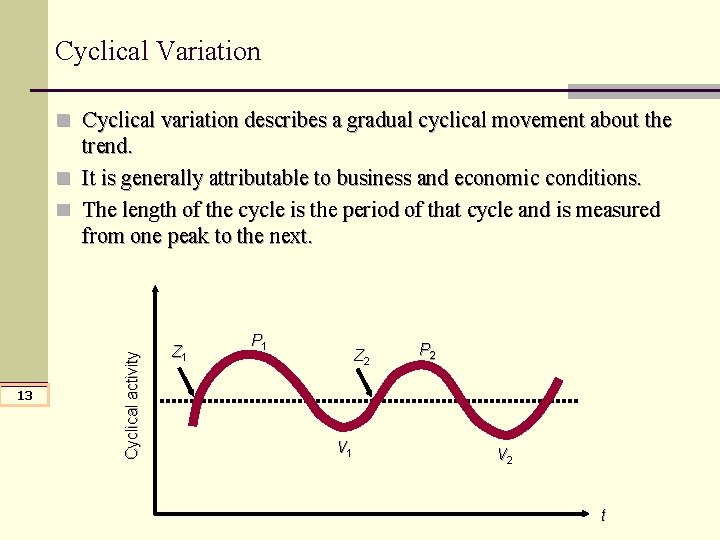
Cyclical Variation n Cyclical variation describes a gradual cyclical movement about the 13 Cyclical activity trend. n It is generally attributable to business and economic conditions. n The length of the cycle is the period of that cycle and is measured from one peak to the next. Z 1 P 1 Z 2 V 1 P 2 V 2 t

Irregular Activity (Noise) n Irregular activity consists of what is “left over” after accounting for the effect of any trend, seasonality, or cyclical activity. 14

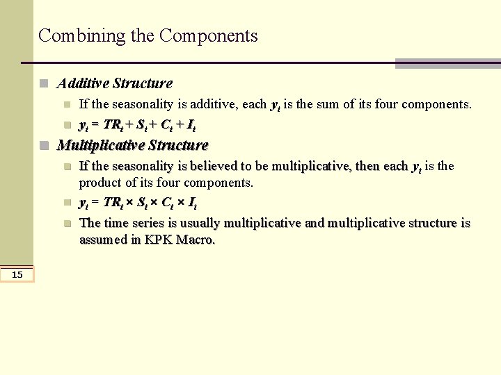
Combining the Components n Additive Structure n If the seasonality is additive, each yt is the sum of its four components. n yt = TRt + St + Ct + It n Multiplicative Structure n If the seasonality is believed to be multiplicative, then each yt is the product of its four components. n yt = TRt × St × Ct × It n The time series is usually multiplicative and multiplicative structure is assumed in KPK Macro. 15

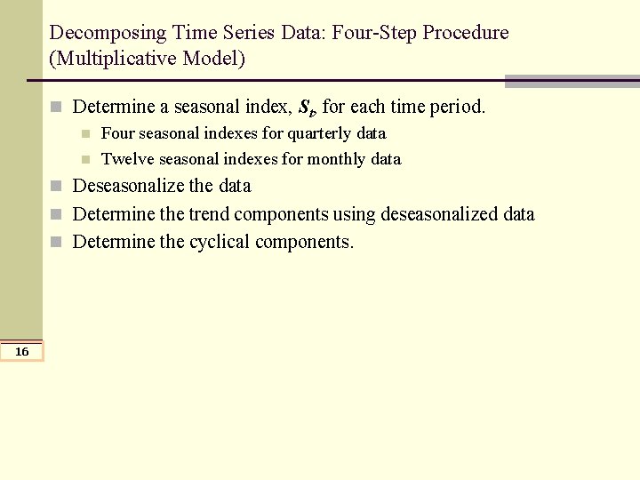
Decomposing Time Series Data: Four-Step Procedure (Multiplicative Model) n Determine a seasonal index, St, for each time period. n Four seasonal indexes for quarterly data n Twelve seasonal indexes for monthly data n Deseasonalize the data n Determine the trend components using deseasonalized data n Determine the cyclical components. 16

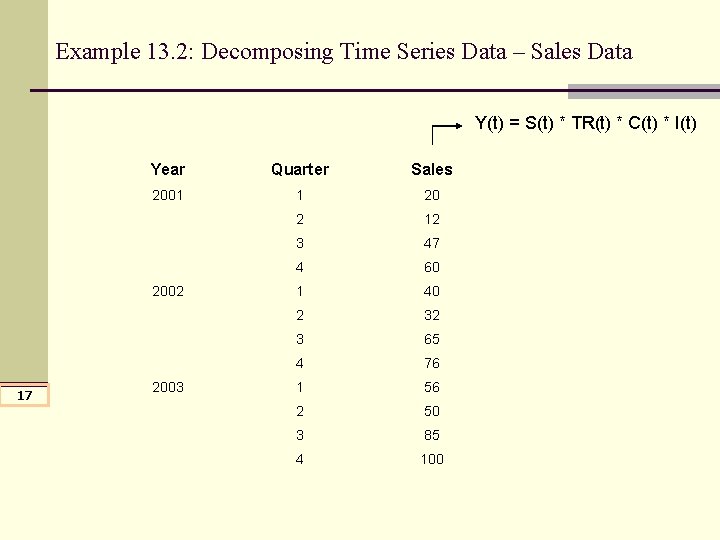
Example 13. 2: Decomposing Time Series Data – Sales Data Y(t) = S(t) * TR(t) * C(t) * I(t) Year Quarter Sales 2001 1 20 2 12 3 47 4 60 1 40 2 32 3 65 4 76 1 56 2 50 3 85 4 100 2002 17 2003

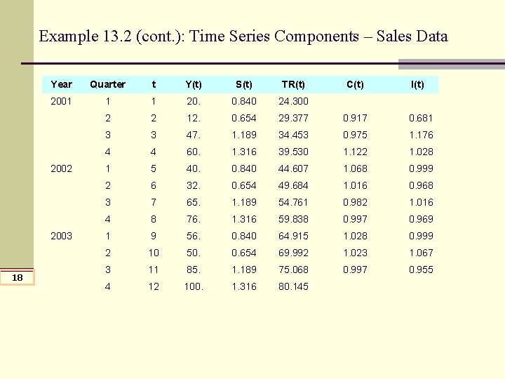
Example 13. 2 (cont. ): Time Series Components – Sales Data Year Quarter t Y(t) S(t) TR(t) 2001 1 1 20. 0. 840 24. 300 2 2 12. 0. 654 29. 377 0. 917 0. 681 3 3 47. 1. 189 34. 453 0. 975 1. 176 4 4 60. 1. 316 39. 530 1. 122 1. 028 1 5 40. 0. 840 44. 607 1. 068 0. 999 2 6 32. 0. 654 49. 684 1. 016 0. 968 3 7 65. 1. 189 54. 761 0. 982 1. 016 4 8 76. 1. 316 59. 838 0. 997 0. 969 1 9 56. 0. 840 64. 915 1. 028 0. 999 2 10 50. 0. 654 69. 992 1. 023 1. 067 3 11 85. 1. 189 75. 068 0. 997 0. 955 4 12 100. 1. 316 80. 145 2002 2003 18 C(t) I(t)

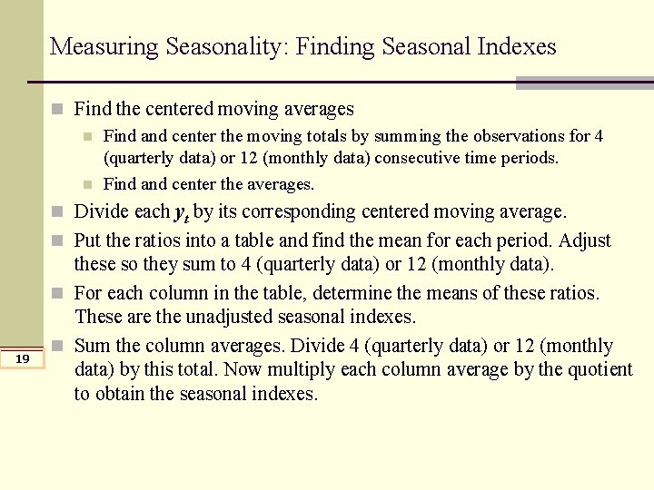
Measuring Seasonality: Finding Seasonal Indexes n Find the centered moving averages n Find and center the moving totals by summing the observations for 4 (quarterly data) or 12 (monthly data) consecutive time periods. n Find and center the averages. n Divide each yt by its corresponding centered moving average. n Put the ratios into a table and find the mean for each period. Adjust 19 these so they sum to 4 (quarterly data) or 12 (monthly data). n For each column in the table, determine the means of these ratios. These are the unadjusted seasonal indexes. n Sum the column averages. Divide 4 (quarterly data) or 12 (monthly data) by this total. Now multiply each column average by the quotient to obtain the seasonal indexes.

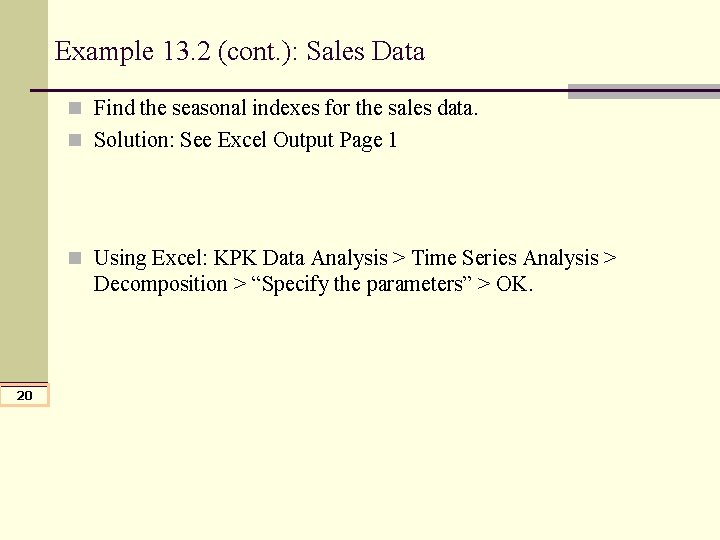
Example 13. 2 (cont. ): Sales Data n Find the seasonal indexes for the sales data. n Solution: See Excel Output Page 1 n Using Excel: KPK Data Analysis > Time Series Analysis > Decomposition > “Specify the parameters” > OK. 20

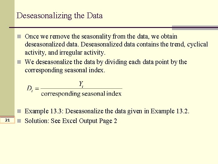
Deseasonalizing the Data n Once we remove the seasonality from the data, we obtain deseasonalized data. Deseasonalized data contains the trend, cyclical activity, and irregular activity. n We deseasonalize the data by dividing each data point by the corresponding seasonal index. n Example 13. 3: Deseasonalize the data given in Example 13. 2. 21 n Solution: See Excel Output Page 2

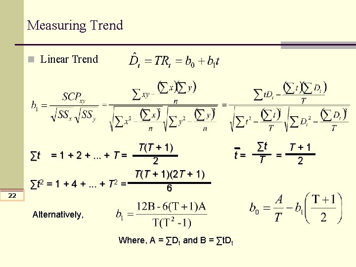
Measuring Trend n Linear Trend 22 T(T + 1) ∑t = 1 + 2 +. . . + T = 2 T(T + 1)(2 T + 1) ∑t 2 = 1 + 4 +. . . + T 2 = 6 Alternatively, Where, A = ∑Dt and B = ∑t. Dt t= ∑t T+1 T = 2

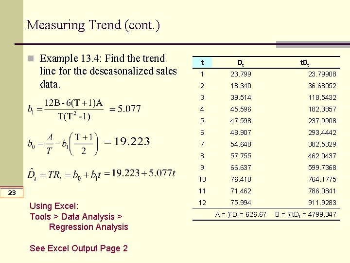
Measuring Trend (cont. ) n Example 13. 4: Find the trend line for the deseasonalized sales data. 23 Using Excel: Tools > Data Analysis > Regression Analysis See Excel Output Page 2 t Dt 1 23. 79908 2 18. 340 36. 68052 3 39. 514 118. 5432 4 45. 596 182. 3857 5 47. 598 237. 9908 6 48. 907 293. 4442 7 54. 648 382. 5329 8 57. 755 462. 0437 9 66. 637 599. 7368 10 76. 418 764. 1775 11 71. 462 786. 0841 12 75. 994 911. 9283 A = ∑Dt = 626. 67 t. Dt B = ∑t. Dt = 4799. 347

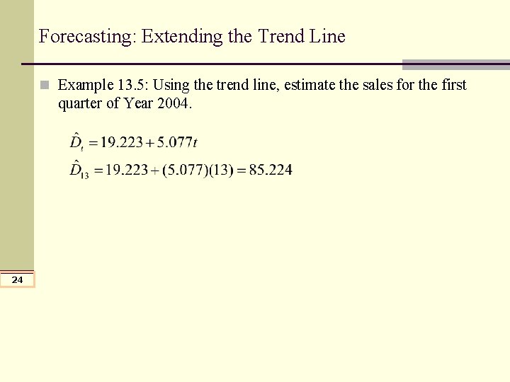
Forecasting: Extending the Trend Line n Example 13. 5: Using the trend line, estimate the sales for the first quarter of Year 2004. 24

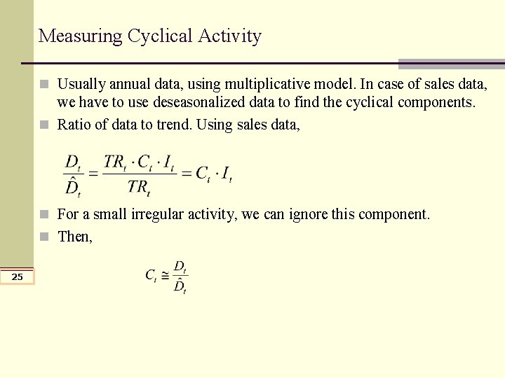
Measuring Cyclical Activity n Usually annual data, using multiplicative model. In case of sales data, we have to use deseasonalized data to find the cyclical components. n Ratio of data to trend. Using sales data, n For a small irregular activity, we can ignore this component. n Then, 25

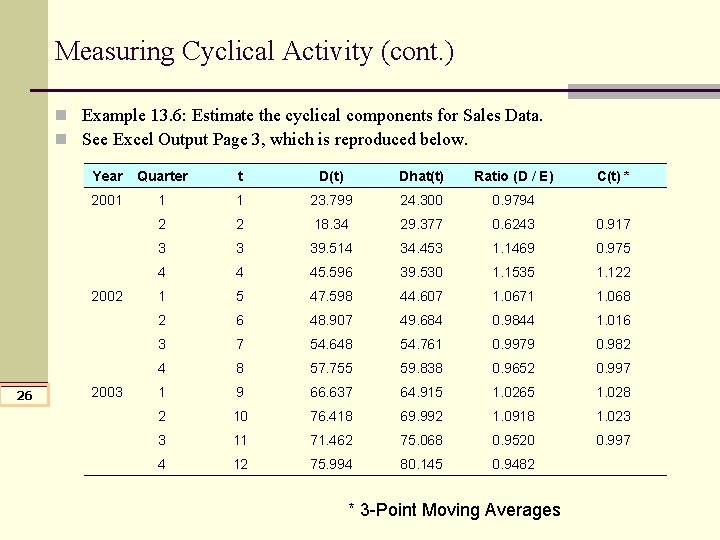
Measuring Cyclical Activity (cont. ) n Example 13. 6: Estimate the cyclical components for Sales Data. n See Excel Output Page 3, which is reproduced below. Year Quarter t D(t) Dhat(t) Ratio (D / E) 2001 1 1 23. 799 24. 300 0. 9794 2 2 18. 34 29. 377 0. 6243 0. 917 3 3 39. 514 34. 453 1. 1469 0. 975 4 4 45. 596 39. 530 1. 1535 1. 122 1 5 47. 598 44. 607 1. 0671 1. 068 2 6 48. 907 49. 684 0. 9844 1. 016 3 7 54. 648 54. 761 0. 9979 0. 982 4 8 57. 755 59. 838 0. 9652 0. 997 1 9 66. 637 64. 915 1. 0265 1. 028 2 10 76. 418 69. 992 1. 0918 1. 023 3 11 71. 462 75. 068 0. 9520 0. 997 4 12 75. 994 80. 145 0. 9482 2002 26 2003 * 3 -Point Moving Averages C(t) *

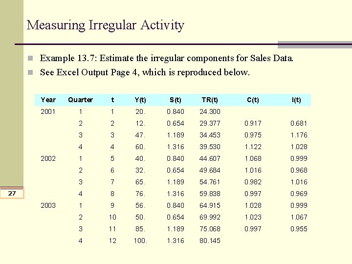
Measuring Irregular Activity n Example 13. 7: Estimate the irregular components for Sales Data. n See Excel Output Page 4, which is reproduced below. Year Quarter t Y(t) S(t) TR(t) 2001 1 1 20. 0. 840 24. 300 2 2 12. 0. 654 29. 377 0. 917 0. 681 3 3 47. 1. 189 34. 453 0. 975 1. 176 4 4 60. 1. 316 39. 530 1. 122 1. 028 1 5 40. 0. 840 44. 607 1. 068 0. 999 2 6 32. 0. 654 49. 684 1. 016 0. 968 3 7 65. 1. 189 54. 761 0. 982 1. 016 4 8 76. 1. 316 59. 838 0. 997 0. 969 1 9 56. 0. 840 64. 915 1. 028 0. 999 2 10 50. 0. 654 69. 992 1. 023 1. 067 3 11 85. 1. 189 75. 068 0. 997 0. 955 4 12 100. 1. 316 80. 145 2002 27 2003 C(t) I(t)

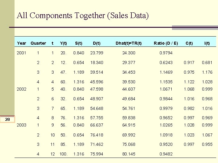
All Components Together (Sales Data) Year Quarter t Y(t) S(t) Dhat(t)=TR(t) Ratio (D / E) 2001 1 1 20. 0. 840 23. 799 24. 300 0. 9794 2 2 12. 0. 654 18. 340 29. 377 3 3 47. 1. 189 39. 514 4 4 60. 1. 316 1 5 40. 2 6 3 2002 28 2003 C(t) I(t) 0. 6243 0. 917 0. 681 34. 453 1. 1469 0. 975 1. 176 45. 596 39. 530 1. 1535 1. 122 1. 028 0. 840 47. 598 44. 607 1. 0671 1. 068 0. 999 32. 0. 654 48. 907 49. 684 0. 9844 1. 016 0. 968 7 65. 1. 189 54. 648 54. 761 0. 9979 0. 982 1. 016 4 8 76. 1. 316 57. 755 59. 838 0. 9652 0. 997 0. 969 1 9 56. 0. 840 66. 637 64. 915 1. 0265 1. 028 0. 999 2 10 50. 0. 654 76. 418 69. 992 1. 0918 1. 023 1. 067 3 11 85. 1. 189 71. 462 75. 068 0. 9520 0. 997 0. 955 4 12 100. 1. 316 75. 994 80. 145 0. 9482

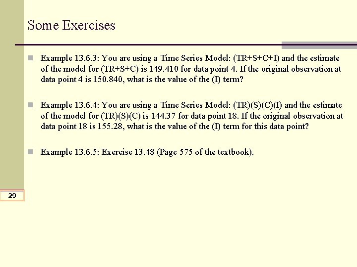
Some Exercises n Example 13. 6. 3: You are using a Time Series Model: (TR+S+C+I) and the estimate of the model for (TR+S+C) is 149. 410 for data point 4. If the original observation at data point 4 is 150. 840, what is the value of the (I) term? n Example 13. 6. 4: You are using a Time Series Model: (TR)(S)(C)(I) and the estimate of the model for (TR)(S)(C) is 144. 37 for data point 18. If the original observation at data point 18 is 155. 28, what is the value of the (I) term for this data point? n Example 13. 6. 5: Exercise 13. 48 (Page 575 of the textbook). 29

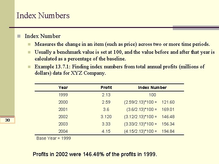
Index Numbers n Index Number n Measures the change in an item (such as price) across two or more time periods. n Usually a benchmark value is set at 100, and the value before and after that year is calculated as a percentage of the baseline. n Example 13. 7. 1: Finding index numbers from total annual profits (millions of dollars) data for XYZ Company. 30 Year Profit Index Number 1999 2. 13 100 2000 2. 59 (2. 59/2. 13)*100 = 121. 60 2001 3. 6 (3. 6/2. 13)*100 = 169. 01 2002 3. 120 (3. 12/2. 13)*100 = 146. 48 2003 3. 33 (3. 33/2. 13)*100 = 156. 34 2004 4. 15 (4. 15/2. 13)*100 = 194. 84 Base Year = 1999 Profits in 2002 were 146. 48% of the profits in 1999.

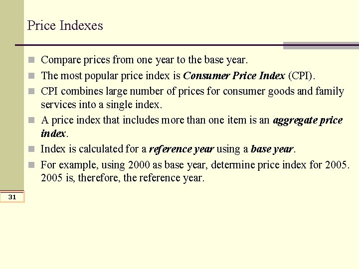
Price Indexes n Compare prices from one year to the base year. n The most popular price index is Consumer Price Index (CPI). n CPI combines large number of prices for consumer goods and family services into a single index. n A price index that includes more than one item is an aggregate price index. n Index is calculated for a reference year using a base year. n For example, using 2000 as base year, determine price index for 2005 is, therefore, the reference year. 31

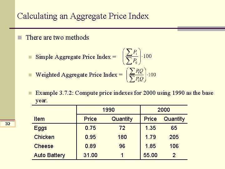
Calculating an Aggregate Price Index n There are two methods n Simple Aggregate Price Index = n Weighted Aggregate Price Index = n Example 3. 7. 2: Compute price indexes for 2000 using 1990 as the base year. 1990 32 2000 Item Price Quantity Eggs 0. 75 72 1. 35 65 Chicken 0. 95 180 1. 79 205 Cheese 0. 89 96 1. 85 106 Auto Battery 31. 00 1 55. 00 2

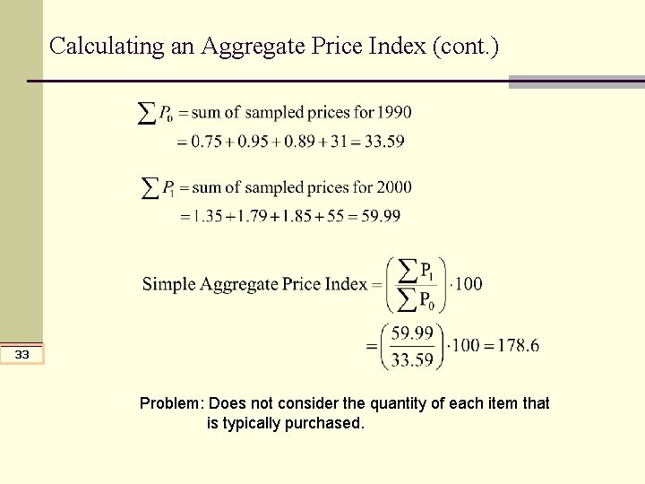
Calculating an Aggregate Price Index (cont. ) 33 Problem: Does not consider the quantity of each item that is typically purchased.

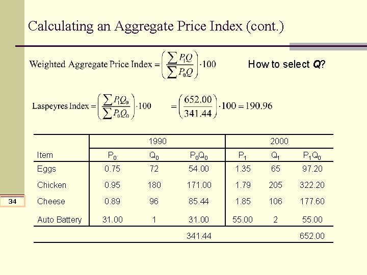
Calculating an Aggregate Price Index (cont. ) How to select Q? 1990 34 2000 Item P 0 Q 0 P 0 Q 0 P 1 Q 1 P 1 Q 0 Eggs 0. 75 72 54. 00 1. 35 65 97. 20 Chicken 0. 95 180 171. 00 1. 79 205 322. 20 Cheese 0. 89 96 85. 44 1. 85 106 177. 60 Auto Battery 31. 00 1 31. 00 55. 00 2 55. 00 341. 44 652. 00

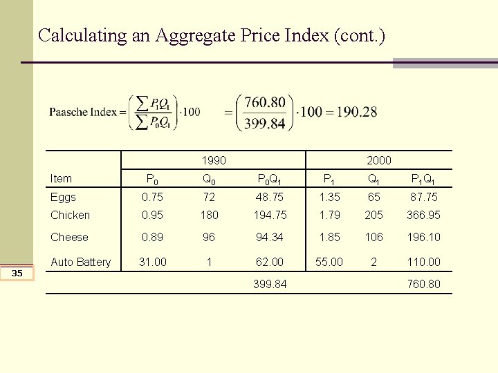
Calculating an Aggregate Price Index (cont. ) 1990 35 2000 Item P 0 Q 0 P 0 Q 1 P 1 Q 1 Eggs 0. 75 72 48. 75 1. 35 65 87. 75 Chicken 0. 95 180 194. 75 1. 79 205 366. 95 Cheese 0. 89 96 94. 34 1. 85 106 196. 10 Auto Battery 31. 00 1 62. 00 55. 00 2 110. 00 399. 84 760. 80