Chapter 13 SUPERVISED LEARNING NEURAL NETWORKS Cios Pedrycz

Chapter 13 SUPERVISED LEARNING: NEURAL NETWORKS Cios / Pedrycz / Swiniarski / Kurgan

Outline • Introduction • Biological Neurons and their Models - Spiking - Simple neuron • Learning Rules - for spiking neurons - for simple neurons • Radial Basis Functions - … - Confidence Measures - RBFs in Knowledge Discovery 2 © 2007 Cios / Pedrycz / Swiniarski / Kurgan

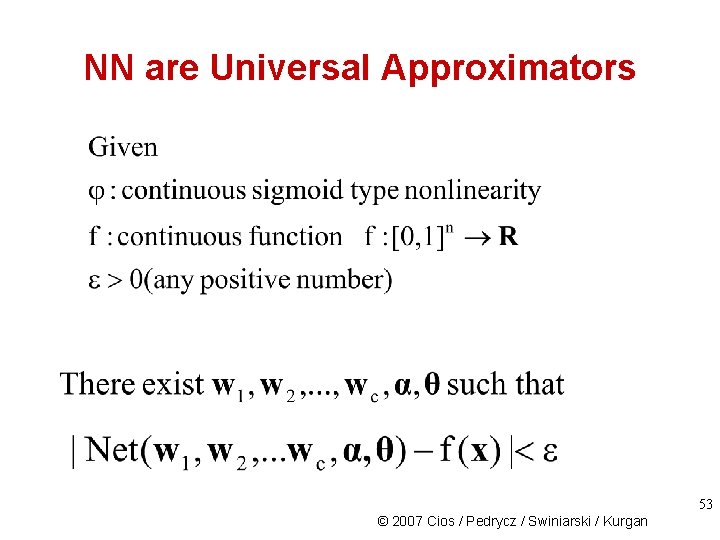
Introduction Interest in artificial neural networks (NN) arose from the realization that the human brain has been and still is the best recognition “device”. NNs are universal approximators, namely, they can approximate any mapping function between known inputs and corresponding known outputs (training data), to any desired degree of accuracy (meaning the error of approximation can be made arbitrarily small). 3 © 2007 Cios / Pedrycz / Swiniarski / Kurgan

Introduction NN characteristics: • learning and generalization ability • fault tolerance • self-organization • robustness • generally, do simple basic calculations Typical application areas: • clustering (SOM) • function approximation • prediction • pattern recognition 4 © 2007 Cios / Pedrycz / Swiniarski / Kurgan

Introduction When to use NN? - Problem requires quantitative knowledge from available data that are often multivariable, noisy, error-prone The phenomena involved are so complex that other approaches are not feasible, or computationally viable Project development time is short (but with enough time for training) “Black-box” nature of neural networks. Learning aspects: • overfitting • learning time and schemes • scaling up properties - 5 © 2007 Cios / Pedrycz / Swiniarski / Kurgan

Introduction To design any type of NN the following key elements must be determined: • the neuron model(s) used for computations • a learning rule, used to update the weights/synapses associated with connections between the neurons in a network • the topology of a network, which determines how the neurons are arranged and interconnected 6 © 2007 Cios / Pedrycz / Swiniarski / Kurgan

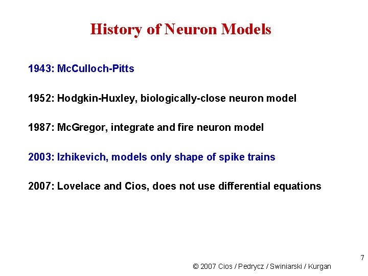
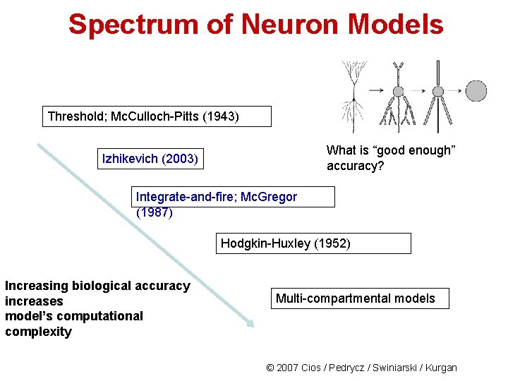
History of Neuron Models 1943: Mc. Culloch-Pitts 1952: Hodgkin-Huxley, biologically-close neuron model 1987: Mc. Gregor, integrate and fire neuron model 2003: Izhikevich, models only shape of spike trains 2007: Lovelace and Cios, does not use differential equations 7 © 2007 Cios / Pedrycz / Swiniarski / Kurgan

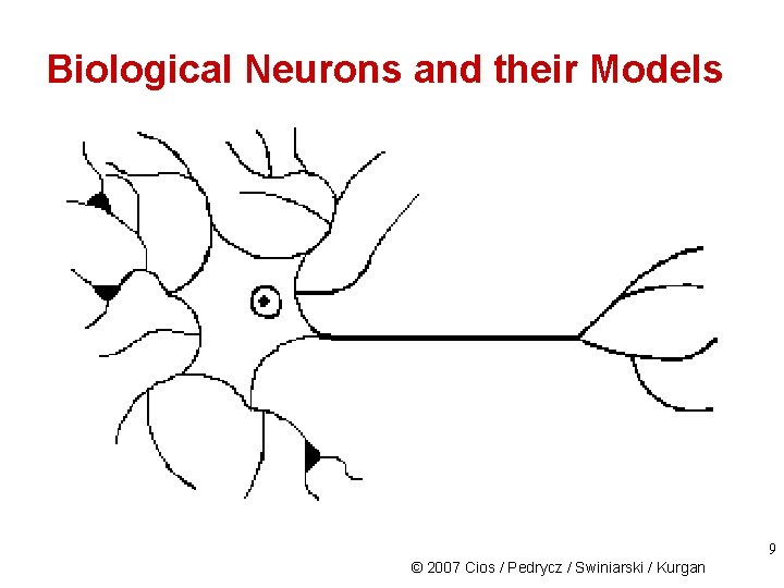
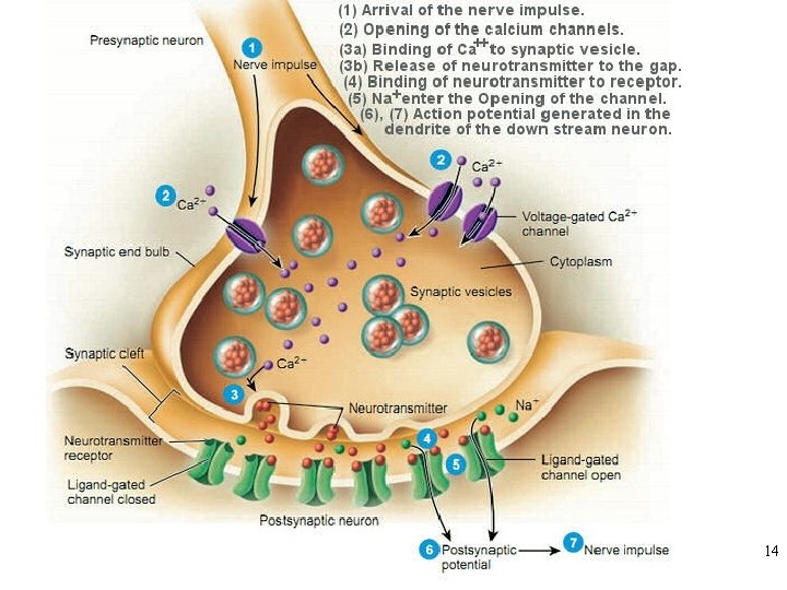
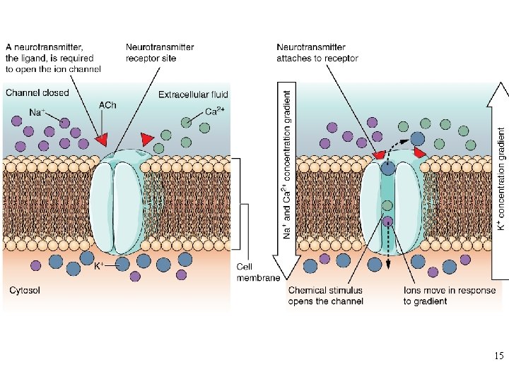
Biological Neurons and their Models All neuron models (aka nodes) resemble biological neurons to some extent. The degree of this resemblance is an important distinguishing factor between different neuron models. The cost of very accurate biological neuron model is high so networks using such neurons usually have only a few thousand neurons. 8 © 2007 Cios / Pedrycz / Swiniarski / Kurgan

Biological Neurons and their Models 9 © 2007 Cios / Pedrycz / Swiniarski / Kurgan

Spectrum of Neuron Models Threshold; Mc. Culloch-Pitts (1943) What is “good enough” accuracy? Izhikevich (2003) Integrate-and-fire; Mc. Gregor (1987) Hodgkin-Huxley (1952) Increasing biological accuracy increases model’s computational complexity Multi-compartmental models © 2007 Cios / Pedrycz / Swiniarski / Kurgan

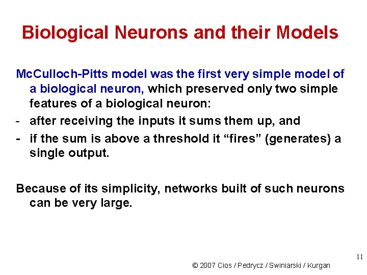
Biological Neurons and their Models Mc. Culloch-Pitts model was the first very simple model of a biological neuron, which preserved only two simple features of a biological neuron: - after receiving the inputs it sums them up, and - if the sum is above a threshold it “fires” (generates) a single output. Because of its simplicity, networks built of such neurons can be very large. 11 © 2007 Cios / Pedrycz / Swiniarski / Kurgan

Mc. Culloch-Pitts 12 © 2007 Cios / Pedrycz / Swiniarski / Kurgan

13

14

15

16

17

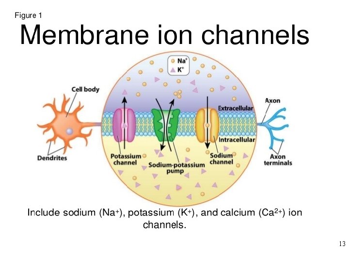
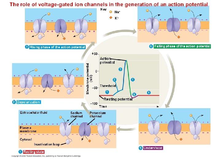
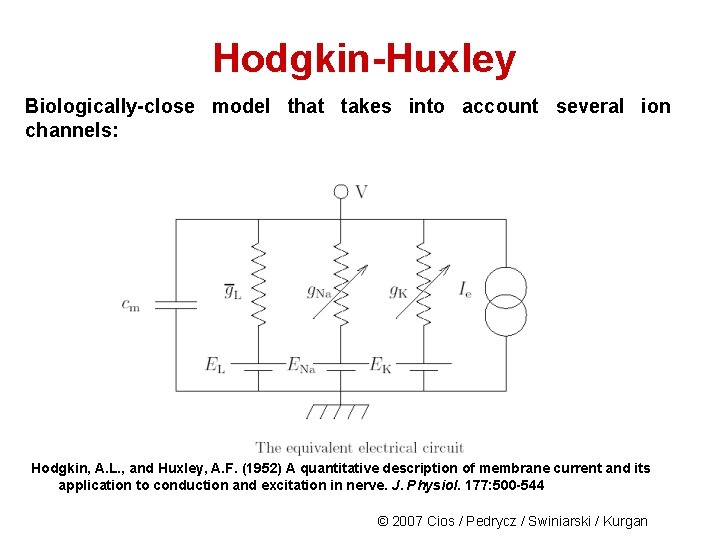
Hodgkin-Huxley Biologically-close model that takes into account several ion channels: Hodgkin, A. L. , and Huxley, A. F. (1952) A quantitative description of membrane current and its application to conduction and excitation in nerve. J. Physiol. 177: 500 -544 © 2007 Cios / Pedrycz / Swiniarski / Kurgan

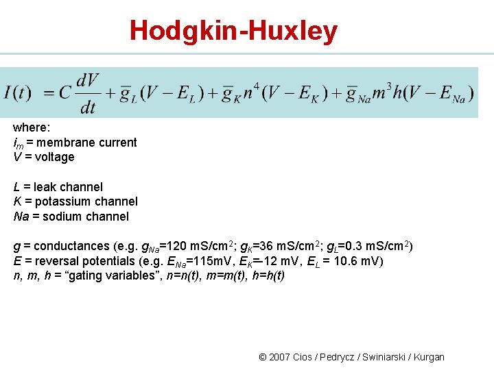
Hodgkin-Huxley where: im = membrane current V = voltage L = leak channel K = potassium channel Na = sodium channel g = conductances (e. g. g. Na=120 m. S/cm 2; g. K=36 m. S/cm 2; g. L=0. 3 m. S/cm 2) E = reversal potentials (e. g. ENa=115 m. V, EK=-12 m. V, EL = 10. 6 m. V) n, m, h = “gating variables”, n=n(t), m=m(t), h=h(t) © 2007 Cios / Pedrycz / Swiniarski / Kurgan

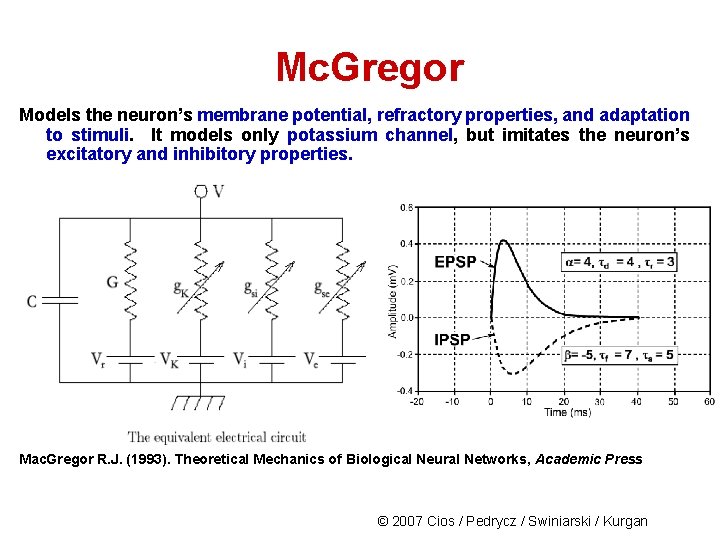
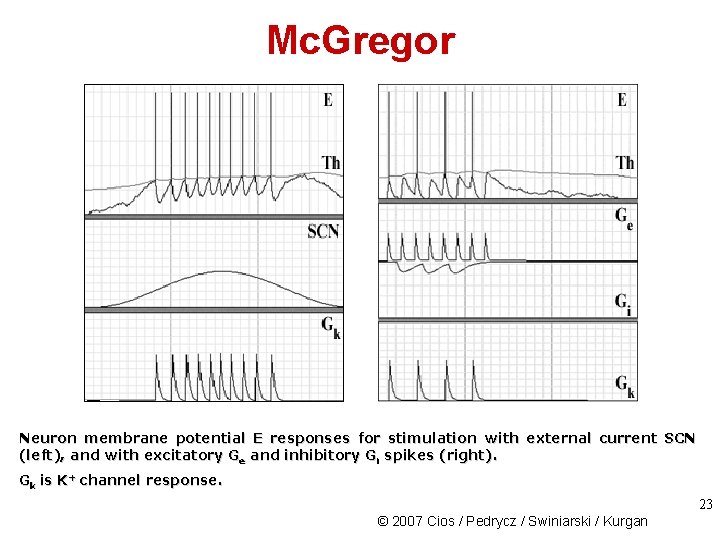
Mc. Gregor Models the neuron’s membrane potential, refractory properties, and adaptation to stimuli. It models only potassium channel, but imitates the neuron’s excitatory and inhibitory properties. Mac. Gregor R. J. (1993). Theoretical Mechanics of Biological Neural Networks, Academic Press © 2007 Cios / Pedrycz / Swiniarski / Kurgan

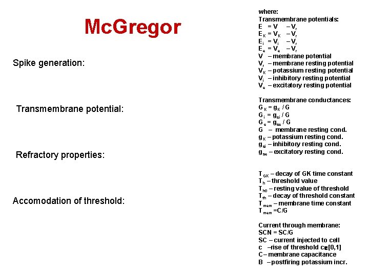
Mc. Gregor Spike generation: Transmembrane potential: Refractory properties: Accomodation of threshold: where: Transmembrane potentials: E = V – Vr EK = V K – V r Ei = V i – V r Ee = V e – V r V – membrane potential Vr – membrane resting potential VK – potassium resting potential Vi – inhibitory resting potential Ve – excitatory resting potential Transmembrane conductances: GK = g K / G Gi = gsi / G Ge = gse / G G – membrane resting cond. g. K – potassium resting cond. gsi – inhibitory resting cond. gse – excitatory resting cond. TGK – decay of GK time constant Th – threshold value Th 0 – resting value of threshold Tth – decay of threshold constant Tmem – membrane time constant Tmem =C/G Current through membrane: SCN = SC/G SC – current injected to cell c –rise of threshold c [0, 1] C– membrane capacitance B – postfiring potassium incr.

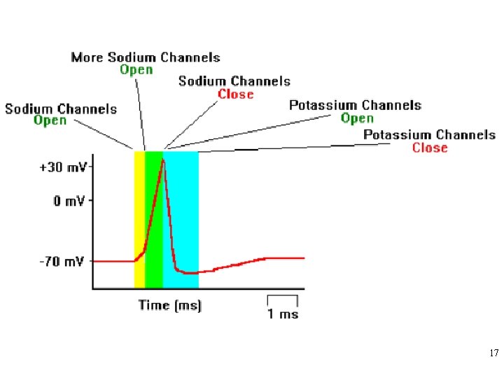
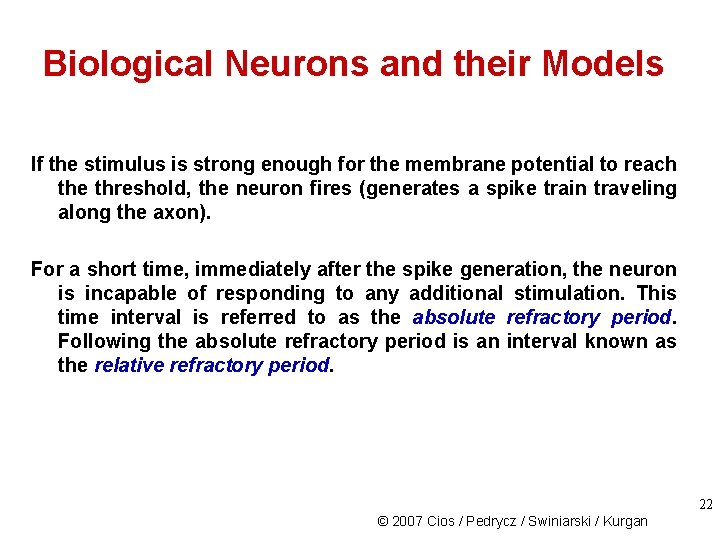
Biological Neurons and their Models If the stimulus is strong enough for the membrane potential to reach the threshold, the neuron fires (generates a spike train traveling along the axon). For a short time, immediately after the spike generation, the neuron is incapable of responding to any additional stimulation. This time interval is referred to as the absolute refractory period. Following the absolute refractory period is an interval known as the relative refractory period. 22 © 2007 Cios / Pedrycz / Swiniarski / Kurgan

Mc. Gregor Neuron membrane potential E responses for stimulation with external current SCN (left), and with excitatory Ge and inhibitory Gi spikes (right). Gk is K+ channel response. 23 © 2007 Cios / Pedrycz / Swiniarski / Kurgan

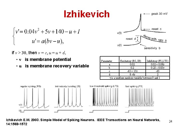
Izhikevich if v > 30, then v = c, u = u + d, • v is membrane potential • u is membrane recovery variable Parameter Excitatory (RS, IB) Inhibitory (FS, LTS) a 0. 02 + 0. 08 b 0. 25 – 0. 05 c -65 + 15 -65 d 8 -6 2 is a uniform random variable between 0 and 1 Izhikevich E. M. 2003. Simple Model of Spiking Neurons. IEEE Transactions on Neural Networks, 14: 1569 -1572 24

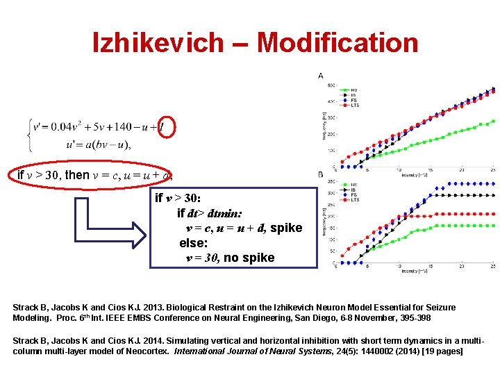
Izhikevich – Modification if v > 30, then v = c, u = u + d, if v > 30: if dt> dtmin: v = c, u = u + d, spike else: v = 30, no spike Strack B, Jacobs K and Cios KJ. 2013. Biological Restraint on the Izhikevich Neuron Model Essential for Seizure Modeling. Proc. 6 th Int. IEEE EMBS Conference on Neural Engineering, San Diego, 6 -8 November, 395 -398 Strack B, Jacobs K and Cios KJ. 2014. Simulating vertical and horizontal inhibition with short term dynamics in a multicolumn multi-layer model of Neocortex. International Journal of Neural Systems, 24(5): 1440002 (2014) [19 pages]

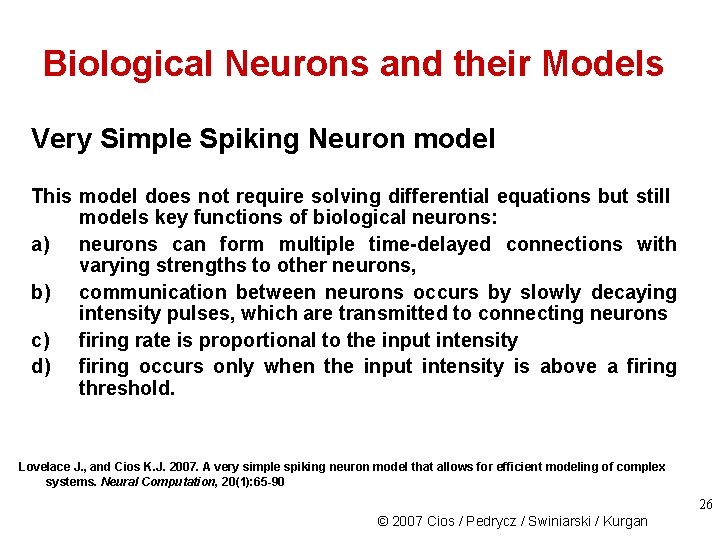
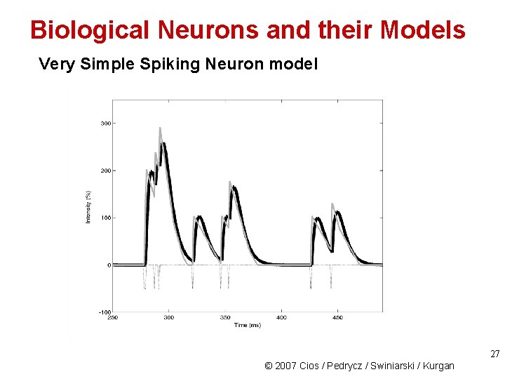
Biological Neurons and their Models Very Simple Spiking Neuron model This model does not require solving differential equations but still models key functions of biological neurons: a) neurons can form multiple time-delayed connections with varying strengths to other neurons, b) communication between neurons occurs by slowly decaying intensity pulses, which are transmitted to connecting neurons c) firing rate is proportional to the input intensity d) firing occurs only when the input intensity is above a firing threshold. Lovelace J. , and Cios K. J. 2007. A very simple spiking neuron model that allows for efficient modeling of complex systems. Neural Computation, 20(1): 65 -90 26 © 2007 Cios / Pedrycz / Swiniarski / Kurgan

Biological Neurons and their Models Very Simple Spiking Neuron model 27 © 2007 Cios / Pedrycz / Swiniarski / Kurgan

Mc. Culloch-Pitts 28 © 2007 Cios / Pedrycz / Swiniarski / Kurgan

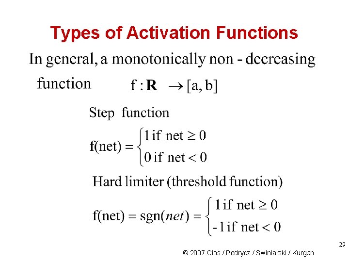
Types of Activation Functions 29 © 2007 Cios / Pedrycz / Swiniarski / Kurgan

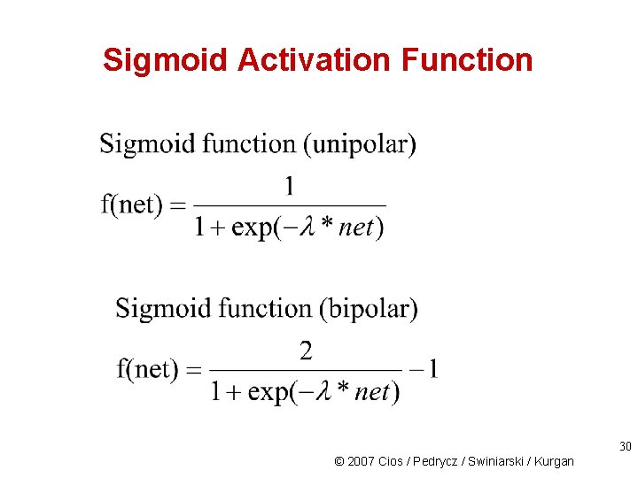
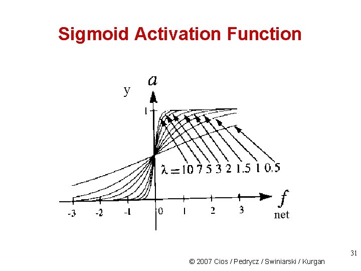
Sigmoid Activation Function 30 © 2007 Cios / Pedrycz / Swiniarski / Kurgan

Sigmoid Activation Function y net 31 © 2007 Cios / Pedrycz / Swiniarski / Kurgan

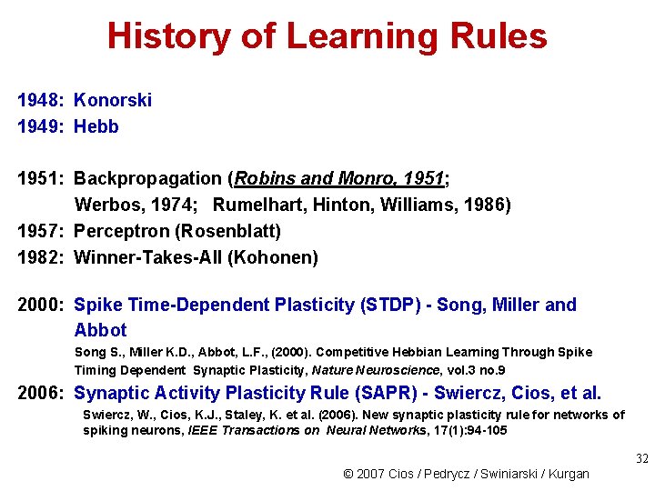
History of Learning Rules 1948: Konorski 1949: Hebb 1951: Backpropagation (Robins and Monro, 1951; Werbos, 1974; Rumelhart, Hinton, Williams, 1986) 1957: Perceptron (Rosenblatt) 1982: Winner-Takes-All (Kohonen) 2000: Spike Time-Dependent Plasticity (STDP) - Song, Miller and Abbot Song S. , Miller K. D. , Abbot, L. F. , (2000). Competitive Hebbian Learning Through Spike Timing Dependent Synaptic Plasticity, Nature Neuroscience, vol. 3 no. 9 2006: Synaptic Activity Plasticity Rule (SAPR) - Swiercz, Cios, et al. Swiercz, W. , Cios, K. J. , Staley, K. et al. (2006). New synaptic plasticity rule for networks of spiking neurons, IEEE Transactions on Neural Networks, 17(1): 94 -105 32 © 2007 Cios / Pedrycz / Swiniarski / Kurgan

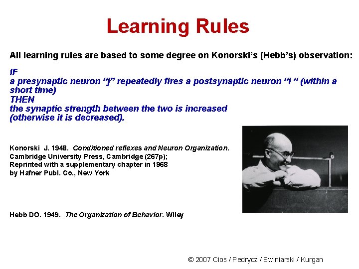
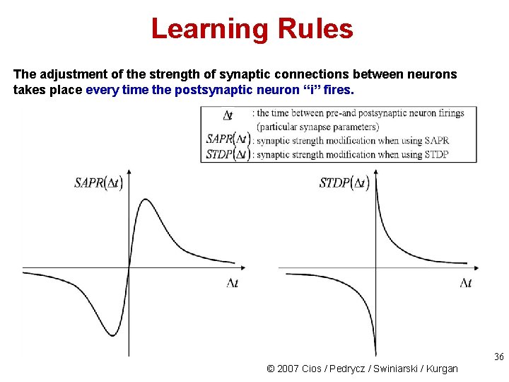
Learning Rules All learning rules are based to some degree on Konorski’s (Hebb’s) observation: IF a presynaptic neuron “j” repeatedly fires a postsynaptic neuron “i “ (within a short time) THEN the synaptic strength between the two is increased (otherwise it is decreased). Konorski J. 1948. Conditioned reflexes and Neuron Organization. Cambridge University Press, Cambridge (267 p); Reprinted with a supplementary chapter in 1968 by Hafner Publ. Co. , New York Hebb DO. 1949. The Organization of Behavior. Wiley © 2007 Cios / Pedrycz / Swiniarski / Kurgan

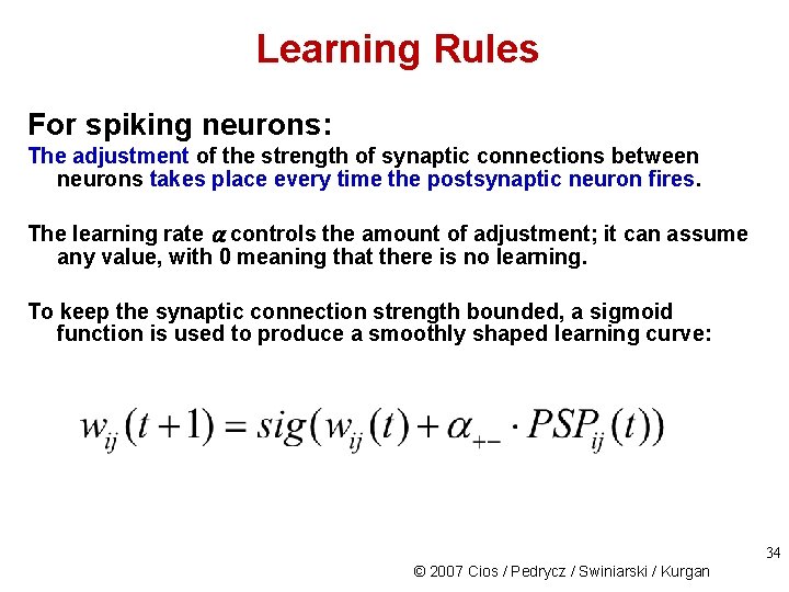
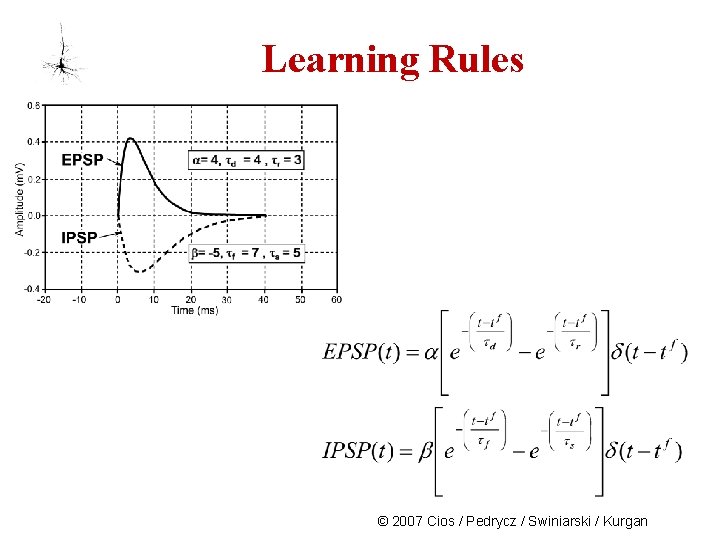
Learning Rules For spiking neurons: The adjustment of the strength of synaptic connections between neurons takes place every time the postsynaptic neuron fires. The learning rate controls the amount of adjustment; it can assume any value, with 0 meaning that there is no learning. To keep the synaptic connection strength bounded, a sigmoid function is used to produce a smoothly shaped learning curve: 34 © 2007 Cios / Pedrycz / Swiniarski / Kurgan

Learning Rules © 2007 Cios / Pedrycz / Swiniarski / Kurgan

Learning Rules The adjustment of the strength of synaptic connections between neurons takes place every time the postsynaptic neuron ‘‘i” fires. 36 © 2007 Cios / Pedrycz / Swiniarski / Kurgan

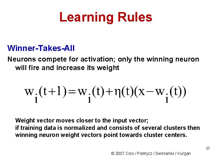
Learning Rules Winner-Takes-All Neurons compete for activation; only the winning neuron will fire and increase its weight Weight vector moves closer to the input vector; if training data is normalized and consists of several clusters then winning neuron weight vectors point towards cluster centers. 37 © 2007 Cios / Pedrycz / Swiniarski / Kurgan

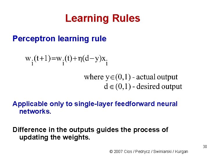
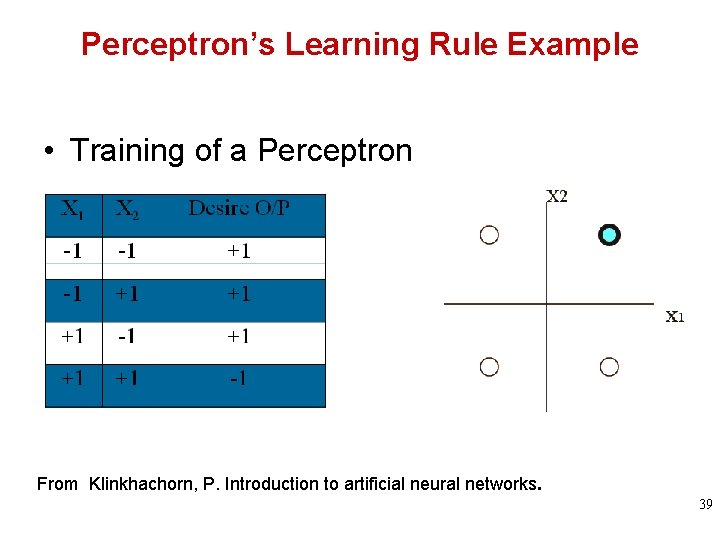
Learning Rules Perceptron learning rule Applicable only to single-layer feedforward neural networks. Difference in the outputs guides the process of updating the weights. 38 © 2007 Cios / Pedrycz / Swiniarski / Kurgan

Perceptron’s Learning Rule Example • Training of a Perceptron From Klinkhachorn, P. Introduction to artificial neural networks. 39

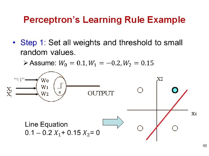
Perceptron’s Learning Rule Example • 40

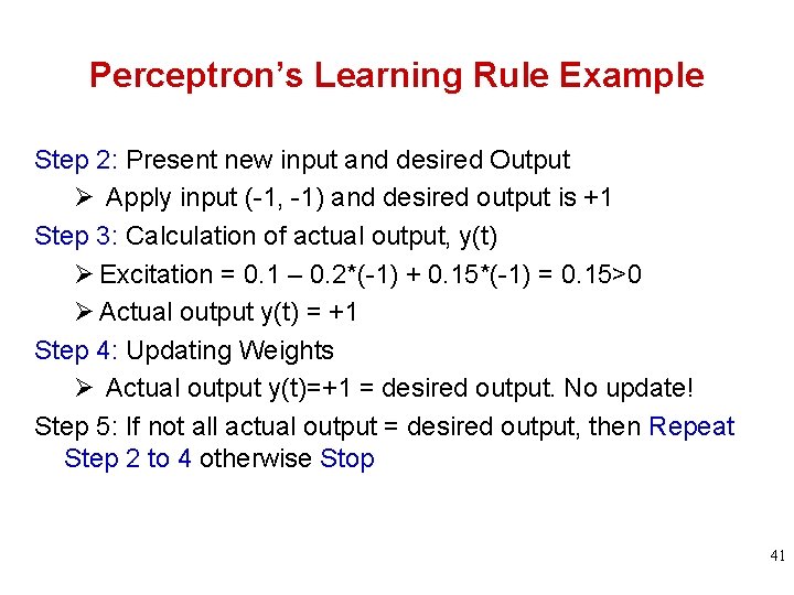
Perceptron’s Learning Rule Example Step 2: Present new input and desired Output Ø Apply input (-1, -1) and desired output is +1 Step 3: Calculation of actual output, y(t) Ø Excitation = 0. 1 – 0. 2*(-1) + 0. 15*(-1) = 0. 15>0 Ø Actual output y(t) = +1 Step 4: Updating Weights Ø Actual output y(t)=+1 = desired output. No update! Step 5: If not all actual output = desired output, then Repeat Step 2 to 4 otherwise Stop 41

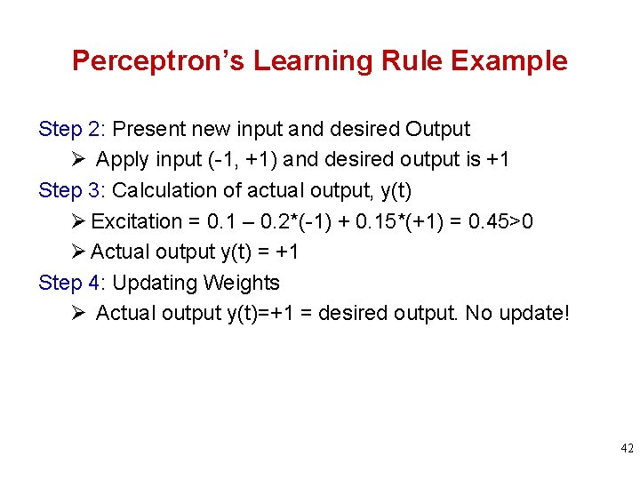
Perceptron’s Learning Rule Example Step 2: Present new input and desired Output Ø Apply input (-1, +1) and desired output is +1 Step 3: Calculation of actual output, y(t) Ø Excitation = 0. 1 – 0. 2*(-1) + 0. 15*(+1) = 0. 45>0 Ø Actual output y(t) = +1 Step 4: Updating Weights Ø Actual output y(t)=+1 = desired output. No update! 42

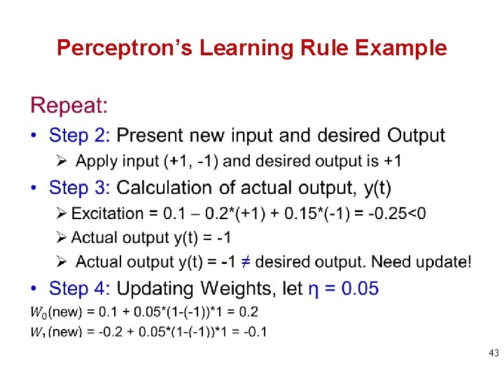
Perceptron’s Learning Rule Example 43

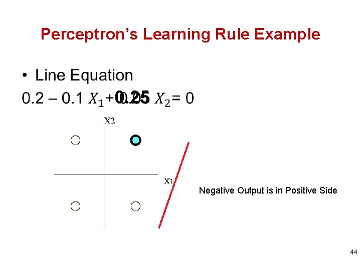
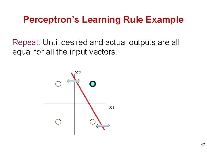
Perceptron’s Learning Rule Example • 0. 25 Negative Output is in Positive Side 44

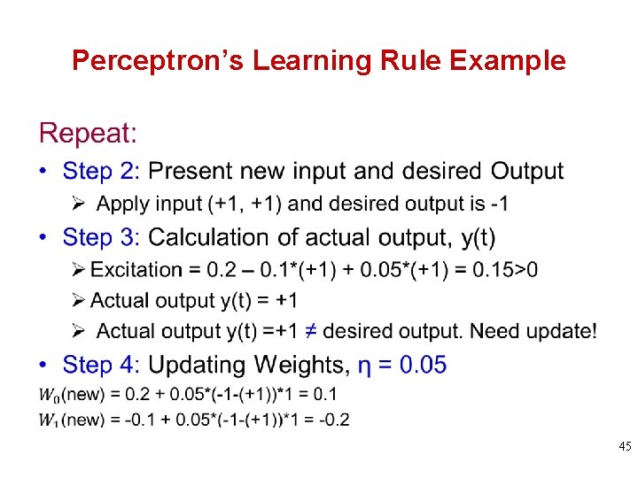
Perceptron’s Learning Rule Example • 45

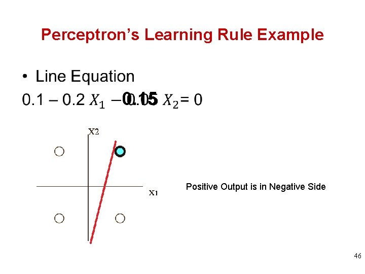
Perceptron’s Learning Rule Example • 0. 15 Positive Output is in Negative Side 46

Perceptron’s Learning Rule Example Repeat: Until desired and actual outputs are all equal for all the input vectors. 47

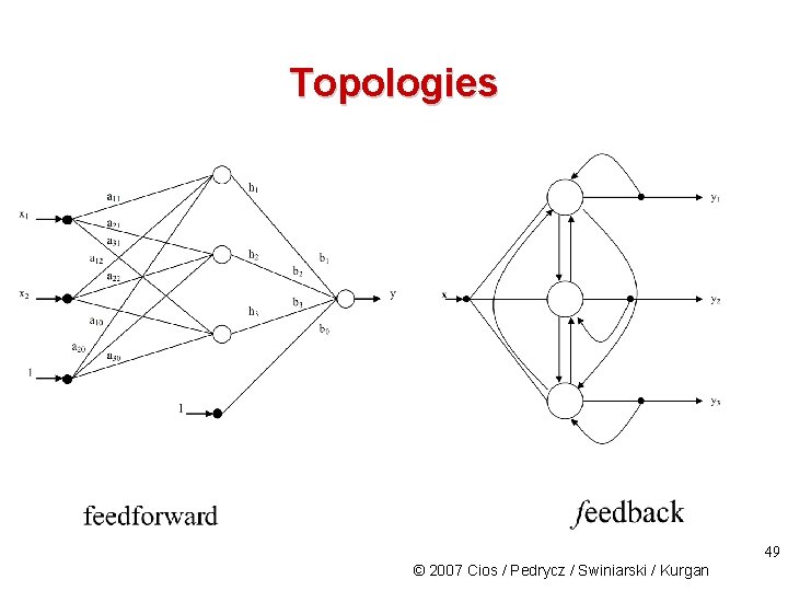
Topology In most cases NN topology has to be specified by the user. The exception is ontogenic NN that generates its own topology on the fly (as needed to solve a problem by adding more nodes and/or layers), using criteria such as an entropy to guide its growth/additions. NN topology can be seen as a directed graph, with neurons being nodes and weighted connections between them the arcs. NN topologies can be divided into two broad categories: • feedforward, with no loops and connections within the same layer Example: Radial Basis Function • recurrent, with possible feedback loops Example: Hopfield 48 © 2007 Cios / Pedrycz / Swiniarski / Kurgan

Topologies 49 © 2007 Cios / Pedrycz / Swiniarski / Kurgan

Feedforward NN Pseudocode Given: Training input-output data pairs, stopping error criterion 1. Select the neuron model 2. Determine the network topology 3. Randomly initialize the NN parameters (weights) 4. Present training data pairs to the network, one by one, and compute the network outputs for each pair 5. For each output that is not correct, adjust the weights, using a chosen learning rule 6. If all output values are below the specified error value then stop; otherwise go to step 4 Result: Trained NN that represents the approximated mapping function y=f(x) 50 © 2007 Cios / Pedrycz / Swiniarski / Kurgan

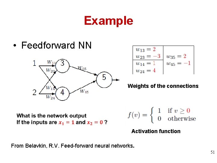
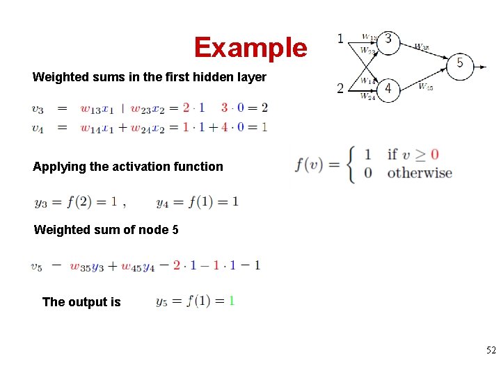
Example • Feedforward NN Weights of the connections Activation function From Belavkin, R. V. Feed-forward neural networks. 51

Example Weighted sums in the first hidden layer Applying the activation function Weighted sum of node 5 The output is 52

NN are Universal Approximators 53 © 2007 Cios / Pedrycz / Swiniarski / Kurgan

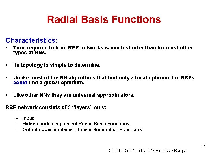
Radial Basis Functions Characteristics: • Time required to train RBF networks is much shorter than for most other types of NNs. • Its topology is simple to determine. • Unlike most of the NN algorithms that find only a local optimum the RBFs could find a global optimum. • Like other NNs they are universal approximators. RBF network consists of 3 “layers” only: – Input – Hidden nodes implement Radial Basis Functions. – Output nodes implement Linear Summation Functions. 54 © 2007 Cios / Pedrycz / Swiniarski / Kurgan

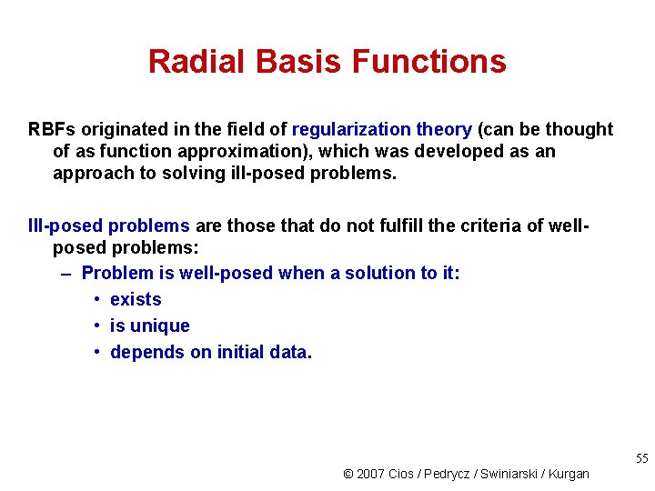
Radial Basis Functions RBFs originated in the field of regularization theory (can be thought of as function approximation), which was developed as an approach to solving ill-posed problems. Ill-posed problems are those that do not fulfill the criteria of wellposed problems: – Problem is well-posed when a solution to it: • exists • is unique • depends on initial data. 55 © 2007 Cios / Pedrycz / Swiniarski / Kurgan

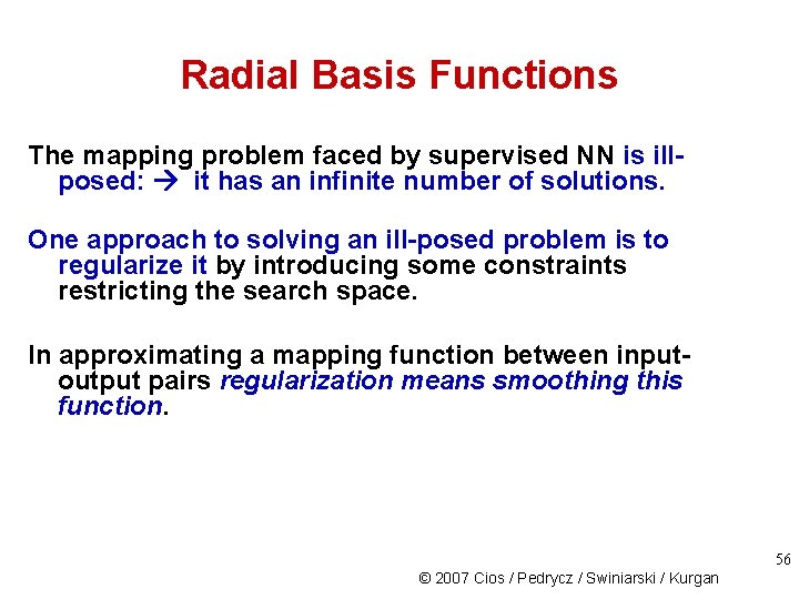
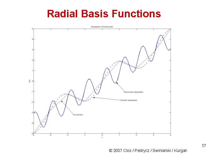
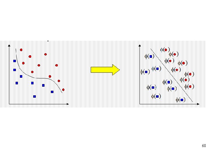
Radial Basis Functions The mapping problem faced by supervised NN is illposed: it has an infinite number of solutions. One approach to solving an ill-posed problem is to regularize it by introducing some constraints restricting the search space. In approximating a mapping function between inputoutput pairs regularization means smoothing this function. 56 © 2007 Cios / Pedrycz / Swiniarski / Kurgan

Radial Basis Functions 57 © 2007 Cios / Pedrycz / Swiniarski / Kurgan

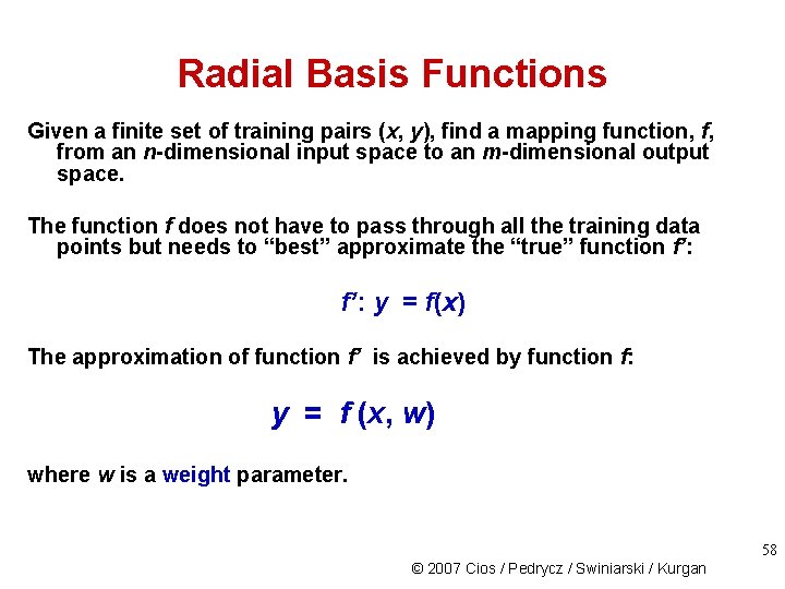
Radial Basis Functions Given a finite set of training pairs (x, y), find a mapping function, f, from an n-dimensional input space to an m-dimensional output space. The function f does not have to pass through all the training data points but needs to “best” approximate the “true” function f’: y = f(x) The approximation of function f’ is achieved by function f: y = f (x, w) where w is a weight parameter. 58 © 2007 Cios / Pedrycz / Swiniarski / Kurgan

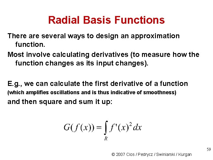
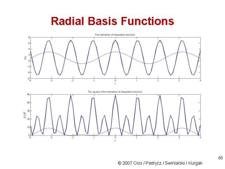
Radial Basis Functions There are several ways to design an approximation function. Most involve calculating derivatives (to measure how the function changes as its input changes). E. g. , we can calculate the first derivative of a function (which amplifies oscillations and is thus indicative of smoothness) and then square and sum it up: 59 © 2007 Cios / Pedrycz / Swiniarski / Kurgan

Radial Basis Functions 60 © 2007 Cios / Pedrycz / Swiniarski / Kurgan

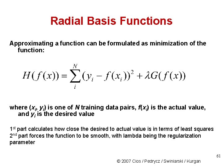
Radial Basis Functions Approximating a function can be formulated as minimization of the function: where (xi, yi) is one of N training data pairs, f(xi) is the actual value, and yi is the desired value 1 st part calculates how close the desired to actual value is in terms of least squares 2 nd part forces the function to be smooth, with lambda being the regularization parameter 61 © 2007 Cios / Pedrycz / Swiniarski / Kurgan

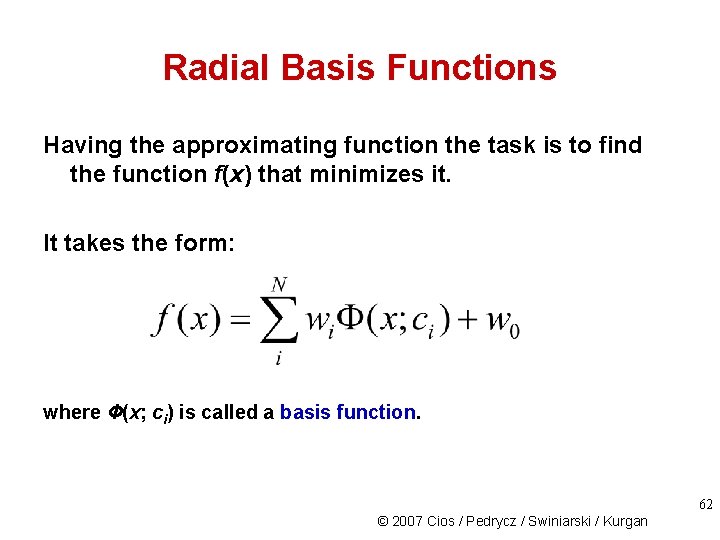
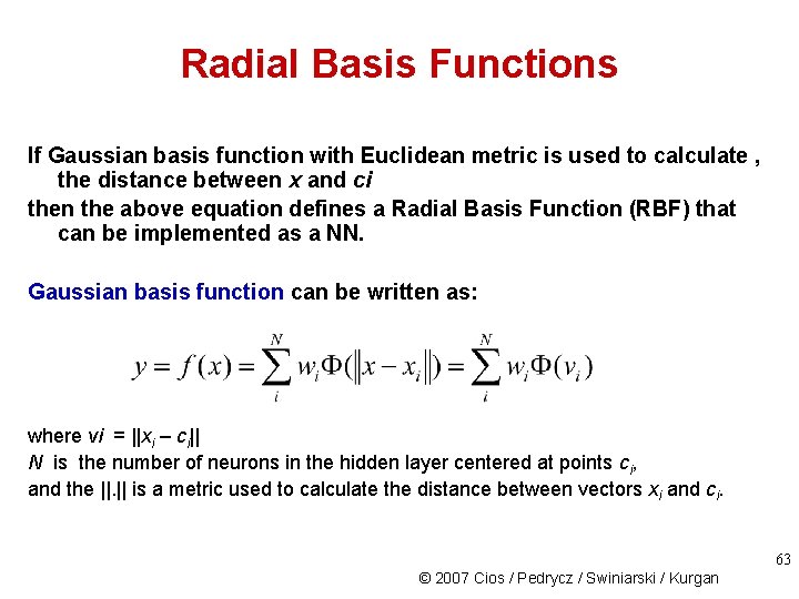
Radial Basis Functions Having the approximating function the task is to find the function f(x) that minimizes it. It takes the form: where Ф(x; ci) is called a basis function. 62 © 2007 Cios / Pedrycz / Swiniarski / Kurgan

Radial Basis Functions If Gaussian basis function with Euclidean metric is used to calculate , the distance between x and ci then the above equation defines a Radial Basis Function (RBF) that can be implemented as a NN. Gaussian basis function can be written as: where vi = ||xi – ci|| N is the number of neurons in the hidden layer centered at points ci, and the ||. || is a metric used to calculate the distance between vectors xi and ci. 63 © 2007 Cios / Pedrycz / Swiniarski / Kurgan

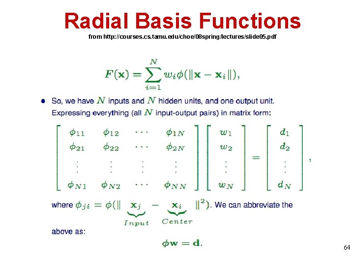
Radial Basis Functions from http: //courses. cs. tamu. edu/choe/08 spring/lectures/slide 05. pdf 64

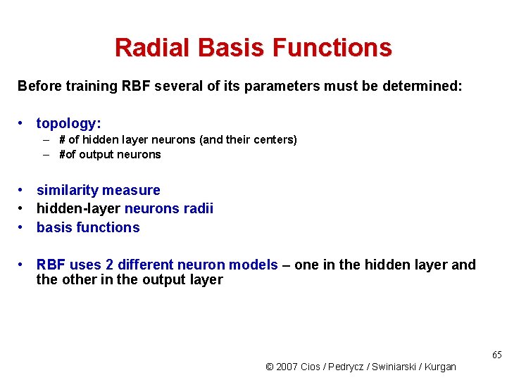
Radial Basis Functions Before training RBF several of its parameters must be determined: • topology: – # of hidden layer neurons (and their centers) – #of output neurons • similarity measure • hidden-layer neurons radii • basis functions • RBF uses 2 different neuron models – one in the hidden layer and the other in the output layer 65 © 2007 Cios / Pedrycz / Swiniarski / Kurgan

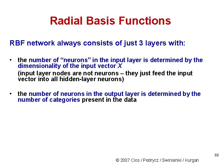
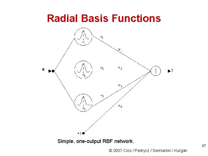
Radial Basis Functions RBF network always consists of just 3 layers with: • the number of “neurons” in the input layer is determined by the dimensionality of the input vector X (input layer nodes are not neurons – they just feed the input vector into all hidden-layer neurons) • the number of neurons in the output layer is determined by the number of categories present in the data 66 © 2007 Cios / Pedrycz / Swiniarski / Kurgan

Radial Basis Functions Simple, one-output RBF network. © 2007 Cios / Pedrycz / Swiniarski / Kurgan 67

68

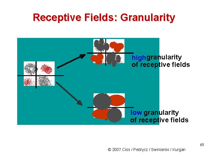
Receptive Fields: Granularity highgranularity of receptive fields low granularity of receptive fields 69 © 2007 Cios / Pedrycz / Swiniarski / Kurgan

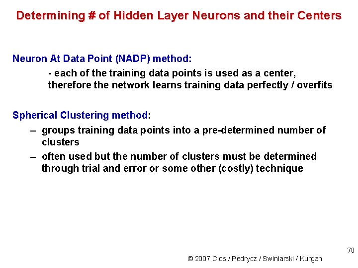
Determining # of Hidden Layer Neurons and their Centers Neuron At Data Point (NADP) method: - each of the training data points is used as a center, therefore the network learns training data perfectly / overfits Spherical Clustering method: – groups training data points into a pre-determined number of clusters – often used but the number of clusters must be determined through trial and error or some other (costly) technique 70 © 2007 Cios / Pedrycz / Swiniarski / Kurgan

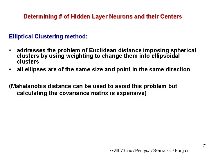
Determining # of Hidden Layer Neurons and their Centers Elliptical Clustering method: • addresses the problem of Euclidean distance imposing spherical clusters by using weighting to change them into ellipsoidal clusters • all ellipses are of the same size and point in the same direction (Mahalanobis distance can be used to avoid this problem but calculating the covariance matrix is expensive) 71 © 2007 Cios / Pedrycz / Swiniarski / Kurgan

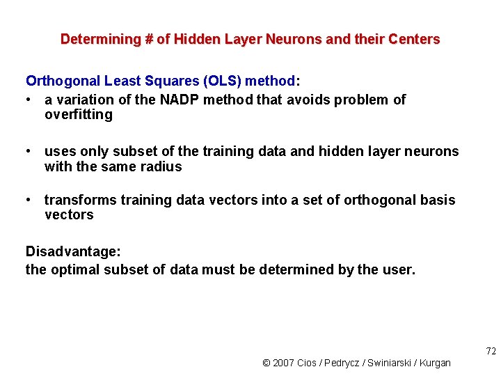
Determining # of Hidden Layer Neurons and their Centers Orthogonal Least Squares (OLS) method: • a variation of the NADP method that avoids problem of overfitting • uses only subset of the training data and hidden layer neurons with the same radius • transforms training data vectors into a set of orthogonal basis vectors Disadvantage: the optimal subset of data must be determined by the user. 72 © 2007 Cios / Pedrycz / Swiniarski / Kurgan

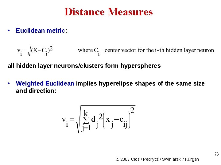
Distance Measures • Euclidean metric: all hidden layer neurons/clusters form hyperspheres • Weighted Euclidean implies hyperelipse shapes of the same size and direction: 73 © 2007 Cios / Pedrycz / Swiniarski / Kurgan

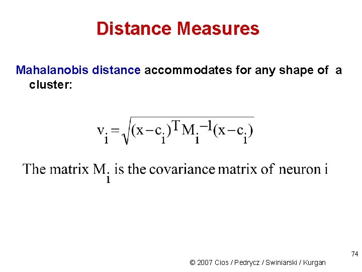
Distance Measures Mahalanobis distance accommodates for any shape of a cluster: 74 © 2007 Cios / Pedrycz / Swiniarski / Kurgan

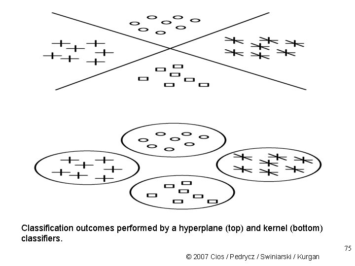
Classification outcomes performed by a hyperplane (top) and kernel (bottom) classifiers. 75 © 2007 Cios / Pedrycz / Swiniarski / Kurgan

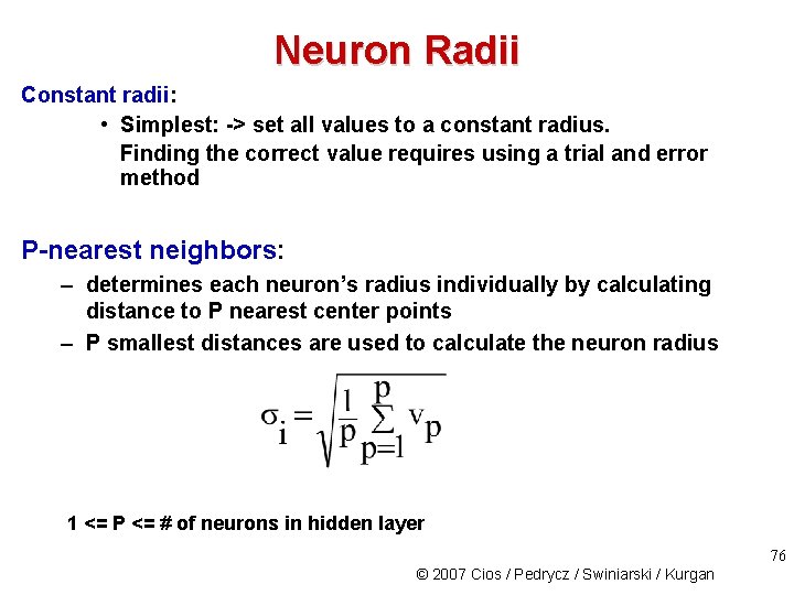
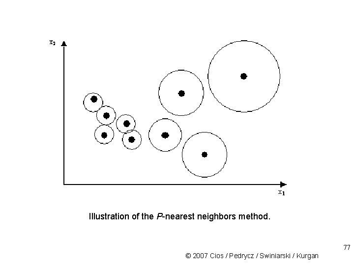
Neuron Radii Constant radii: • Simplest: -> set all values to a constant radius. Finding the correct value requires using a trial and error method P-nearest neighbors: – determines each neuron’s radius individually by calculating distance to P nearest center points – P smallest distances are used to calculate the neuron radius 1 <= P <= # of neurons in hidden layer 76 © 2007 Cios / Pedrycz / Swiniarski / Kurgan

Illustration of the P-nearest neighbors method. 77 © 2007 Cios / Pedrycz / Swiniarski / Kurgan

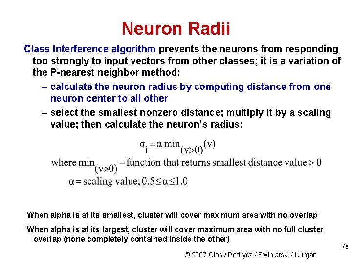
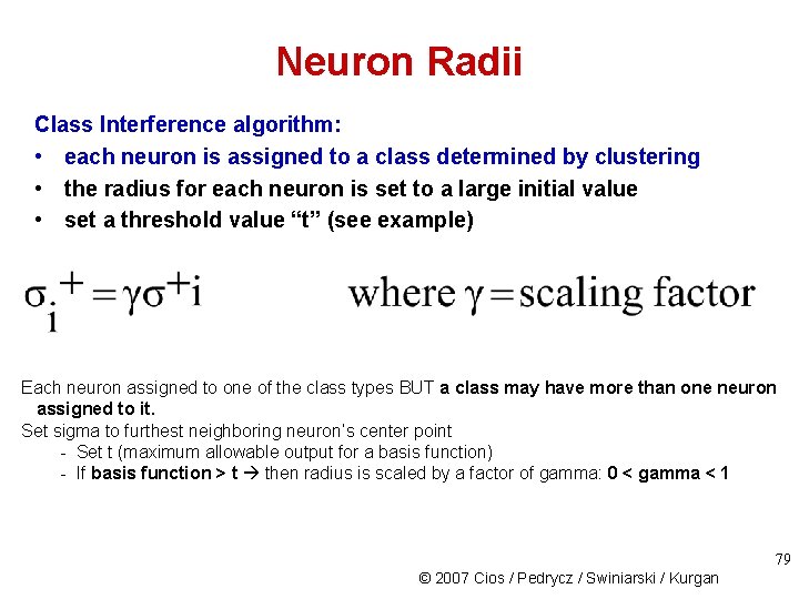
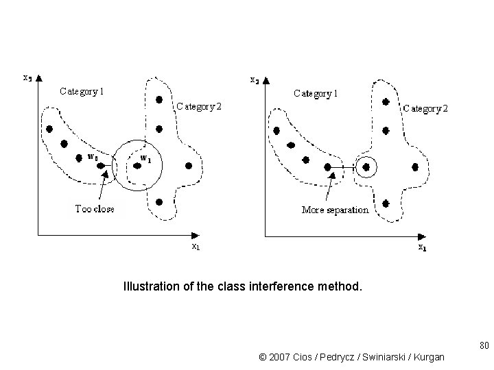
Neuron Radii Class Interference algorithm prevents the neurons from responding too strongly to input vectors from other classes; it is a variation of the P-nearest neighbor method: – calculate the neuron radius by computing distance from one neuron center to all other – select the smallest nonzero distance; multiply it by a scaling value; then calculate the neuron’s radius: When alpha is at its smallest, cluster will cover maximum area with no overlap When alpha is at its largest, cluster will cover maximum area with no full cluster overlap (none completely contained inside the other) © 2007 Cios / Pedrycz / Swiniarski / Kurgan 78

Neuron Radii Class Interference algorithm: • each neuron is assigned to a class determined by clustering • the radius for each neuron is set to a large initial value • set a threshold value “t” (see example) Each neuron assigned to one of the class types BUT a class may have more than one neuron assigned to it. Set sigma to furthest neighboring neuron’s center point - Set t (maximum allowable output for a basis function) - If basis function > t then radius is scaled by a factor of gamma: 0 < gamma < 1 79 © 2007 Cios / Pedrycz / Swiniarski / Kurgan

Illustration of the class interference method. 80 © 2007 Cios / Pedrycz / Swiniarski / Kurgan

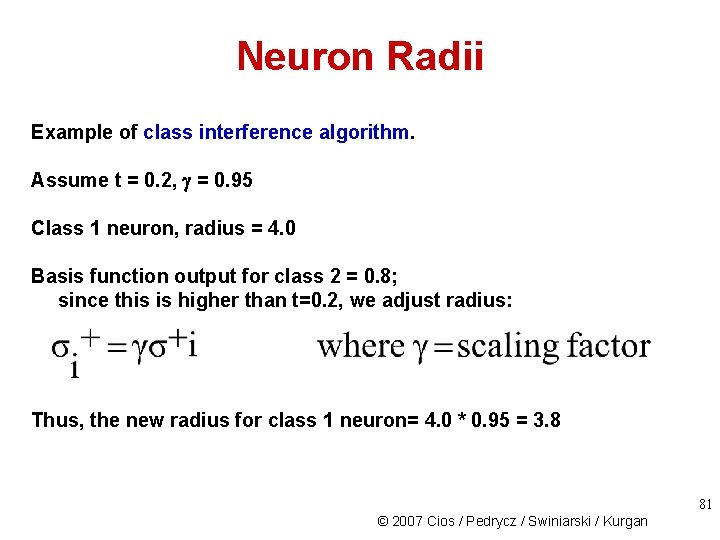
Neuron Radii Example of class interference algorithm. Assume t = 0. 2, = 0. 95 Class 1 neuron, radius = 4. 0 Basis function output for class 2 = 0. 8; since this is higher than t=0. 2, we adjust radius: Thus, the new radius for class 1 neuron= 4. 0 * 0. 95 = 3. 8 81 © 2007 Cios / Pedrycz / Swiniarski / Kurgan

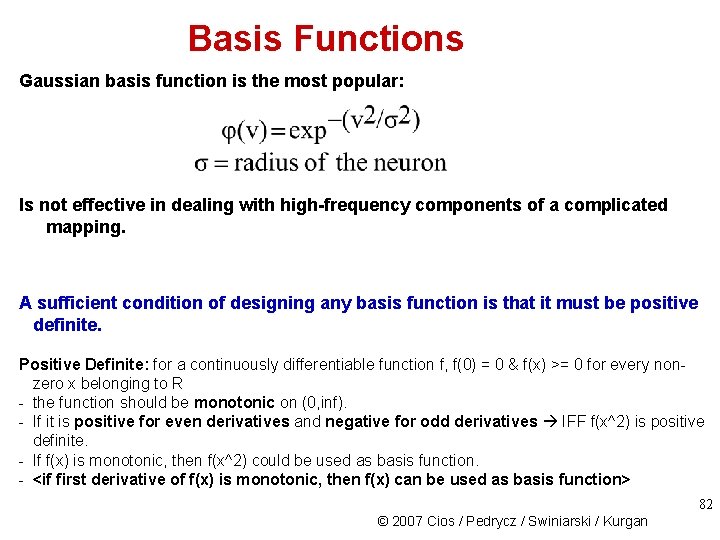
Basis Functions Gaussian basis function is the most popular: Is not effective in dealing with high-frequency components of a complicated mapping. A sufficient condition of designing any basis function is that it must be positive definite. Positive Definite: for a continuously differentiable function f, f(0) = 0 & f(x) >= 0 for every nonzero x belonging to R - the function should be monotonic on (0, inf). - If it is positive for even derivatives and negative for odd derivatives IFF f(x^2) is positive definite. - If f(x) is monotonic, then f(x^2) could be used as basis function. - <if first derivative of f(x) is monotonic, then f(x) can be used as basis function> 82 © 2007 Cios / Pedrycz / Swiniarski / Kurgan

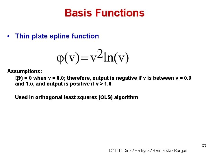
Basis Functions • Thin plate spline function Assumptions: � (v) = 0 when v = 0. 0; therefore, output is negative if v is between v = 0. 0 and 1. 0, and output is positive if v > 1. 0 Used in orthogonal least squares (OLS) algorithm 83 © 2007 Cios / Pedrycz / Swiniarski / Kurgan

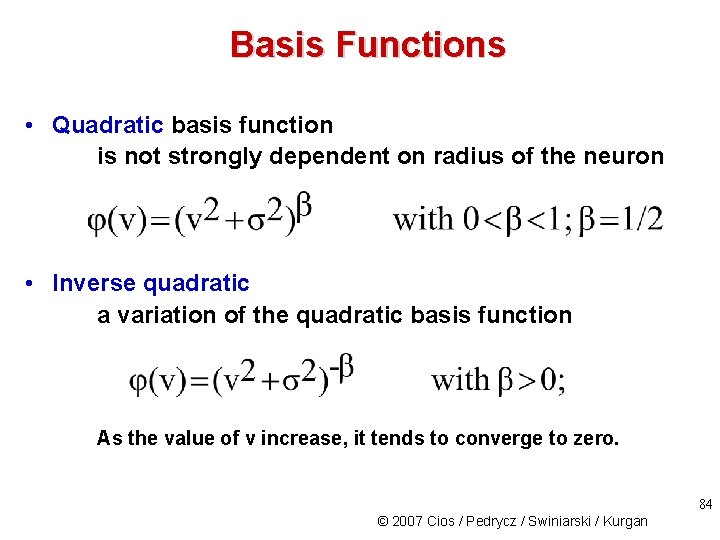
Basis Functions • Quadratic basis function is not strongly dependent on radius of the neuron • Inverse quadratic a variation of the quadratic basis function As the value of v increase, it tends to converge to zero. 84 © 2007 Cios / Pedrycz / Swiniarski / Kurgan

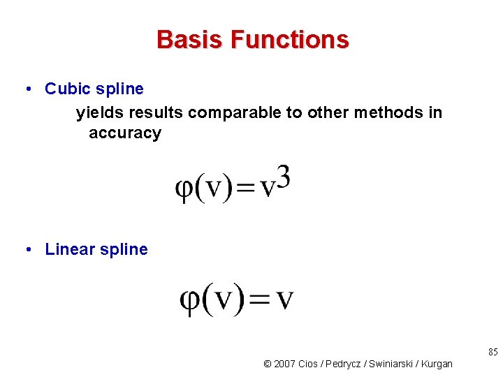
Basis Functions • Cubic spline yields results comparable to other methods in accuracy • Linear spline 85 © 2007 Cios / Pedrycz / Swiniarski / Kurgan

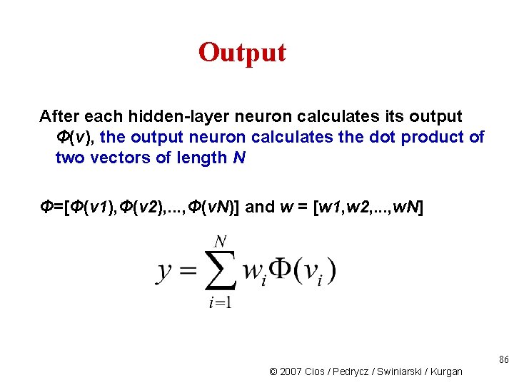
Output After each hidden-layer neuron calculates its output Φ(v), the output neuron calculates the dot product of two vectors of length N Φ=[Φ(v 1), Φ(v 2), . . . , Φ(v. N)] and w = [w 1, w 2, . . . , w. N] 86 © 2007 Cios / Pedrycz / Swiniarski / Kurgan

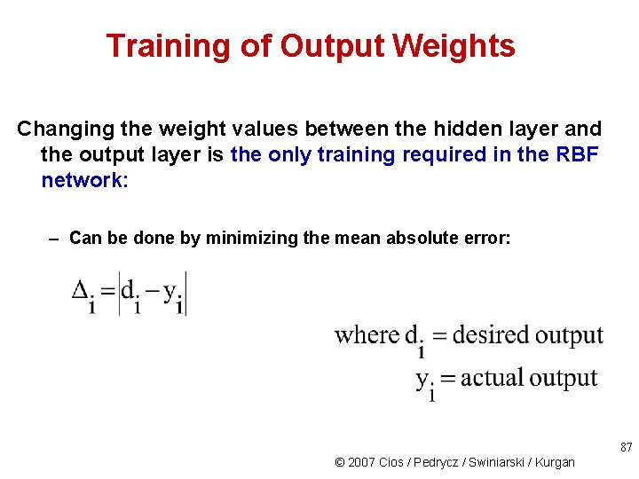
Training of Output Weights Changing the weight values between the hidden layer and the output layer is the only training required in the RBF network: – Can be done by minimizing the mean absolute error: 87 © 2007 Cios / Pedrycz / Swiniarski / Kurgan

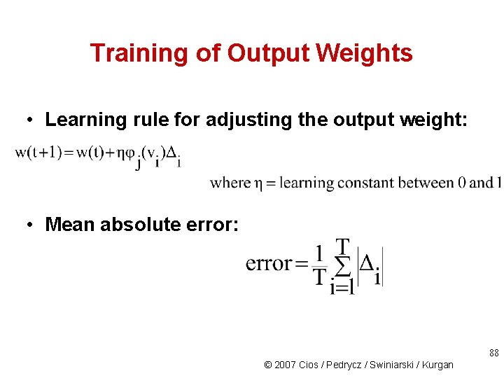
Training of Output Weights • Learning rule for adjusting the output weight: • Mean absolute error: 88 © 2007 Cios / Pedrycz / Swiniarski / Kurgan

Neuron Models Two different neuron models are used in RBF networks: one in the hidden layer and another one in the output layer The first one is determined by the type of the basis function used (most often Gaussian), and the metric used to calculate the distance between the input vector and the hidden-layer center. 89 © 2007 Cios / Pedrycz / Swiniarski / Kurgan

Neuron Models The neuron model used in the output layer can be linear (i. e. , it sums up the outputs of the hidden layer multiplied by the weights to produce the output) or sigmoidal (i. e. , produces output in the range 0 -1). The sigmoidal type of an output layer neuron is used for classification problems, where during training the outputs are trained to be either 0 or 1 (in practice, 0. 1 and 0. 9, to shorten the training time). 90 © 2007 Cios / Pedrycz / Swiniarski / Kurgan

RBF Algorithm Given: Training data pairs, stopping error criteria, sigmoidal neuron model, Gaussian basis function with Euclidean metric 1. determine the network topology 2. choose the neuron model and radii 3. randomly initialize the weights between the hidden and the output layer neurons 4. present the input vector, x, to all hidden layer neurons 5. each hidden layer computes the distance between x and its center point 91 © 2007 Cios / Pedrycz / Swiniarski / Kurgan

RBF Algorithm 6. each hidden layer neuron calculates its basis function output Φ(v) 7. each Φ(v) is multiplied by a weight value and is fed to the output neuron(s) 8. The output neuron(s) sums all the values and outputs the sum as the answer 9. For each output that is not correct, adjust the weights using a learning rule 10. if all the output values are below the specified error value, then stop. Otherwise go to step 8 11. repeat steps 4 through 9 for all remaining training data pairs Result: Trained RBF network 92 © 2007 Cios / Pedrycz / Swiniarski / Kurgan

Radii and centers of three hidden-layer neurons, and two test points x 1 and x 2. 93 © 2007 Cios / Pedrycz / Swiniarski / Kurgan

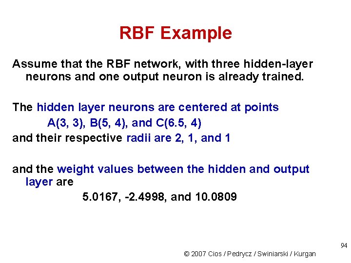
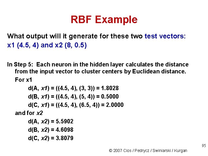
RBF Example Assume that the RBF network, with three hidden-layer neurons and one output neuron is already trained. The hidden layer neurons are centered at points A(3, 3), B(5, 4), and C(6. 5, 4) and their respective radii are 2, 1, and 1 and the weight values between the hidden and output layer are 5. 0167, -2. 4998, and 10. 0809 94 © 2007 Cios / Pedrycz / Swiniarski / Kurgan

RBF Example What output will it generate for these two test vectors: x 1 (4. 5, 4) and x 2 (8, 0. 5) In Step 5: Each neuron in the hidden layer calculates the distance from the input vector to cluster centers by Euclidean distance. For x 1 d(A, x 1) = ((4. 5, 4), (3, 3)) = 1. 8028 d(B, x 1) = ((4. 5, 4), (5, 4)) = 0. 5000 d(C, x 1) = ((4. 5, 4), (6. 5, 4)) = 2. 0000 and for x 2 d(A, x 2) = 5. 5902 d(B, x 2) = 4. 6098 d(C, x 2) = 3. 8079 95 © 2007 Cios / Pedrycz / Swiniarski / Kurgan

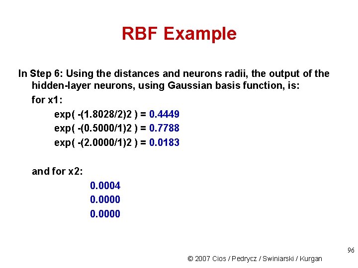
RBF Example In Step 6: Using the distances and neurons radii, the output of the hidden-layer neurons, using Gaussian basis function, is: for x 1: exp( -(1. 8028/2)2 ) = 0. 4449 exp( -(0. 5000/1)2 ) = 0. 7788 exp( -(2. 0000/1)2 ) = 0. 0183 and for x 2: 0. 0004 0. 0000 96 © 2007 Cios / Pedrycz / Swiniarski / Kurgan

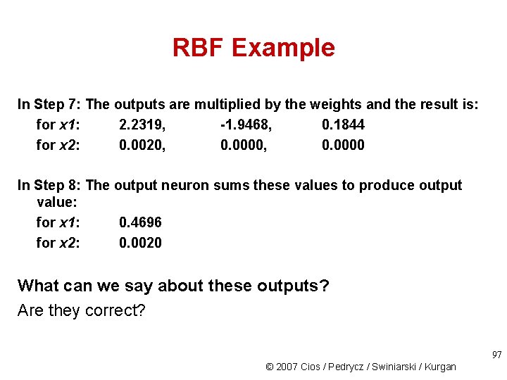
RBF Example In Step 7: The outputs are multiplied by the weights and the result is: for x 1: 2. 2319, -1. 9468, 0. 1844 for x 2: 0. 0020, 0. 0000 In Step 8: The output neuron sums these values to produce output value: for x 1: 0. 4696 for x 2: 0. 0020 What can we say about these outputs? Are they correct? 97 © 2007 Cios / Pedrycz / Swiniarski / Kurgan

Confidence Measures RBF networks, like other supervised NNs, give good results for unseen input data that are similar to any of the data points used in training but give poor results for unfamiliar (very different) input data. • Confidence measures (CM) are used for flagging such unfamiliar data points • Using CM may increase overall accuracy of the network • Some CMs: - Parzen windows (estimates density of an unknown probability distribution function; see Chapter 11) - Certainty factors 98 © 2007 Cios / Pedrycz / Swiniarski / Kurgan

RBF network with reliability measure output 99 © 2007 Cios / Pedrycz / Swiniarski / Kurgan

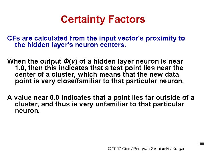
Certainty Factors CFs are calculated from the input vector's proximity to the hidden layer's neuron centers. When the output Φ(v) of a hidden layer neuron is near 1. 0, then this indicates that a test point lies near the center of a cluster, which means that the new data point is very close/familiar to that particular neuron. A value near 0. 0 indicates that a point lies far outside of a cluster, and thus is very unfamiliar to that particular neuron. 100 © 2007 Cios / Pedrycz / Swiniarski / Kurgan

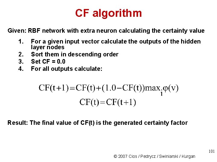
CF algorithm Given: RBF network with extra neuron calculating the certainty value 1. 2. 3. 4. For a given input vector calculate the outputs of the hidden layer nodes Sort them in descending order Set CF = 0. 0 For all outputs calculate: Result: The final value of CF(t) is the generated certainty factor 101 © 2007 Cios / Pedrycz / Swiniarski / Kurgan

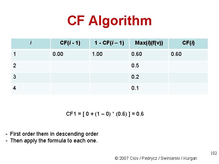
CF Algorithm i 1 CF(i - 1) 0. 00 1 - CF(i – 1) 1. 00 Max(i)(f(v)) 0. 60 2 0. 5 3 0. 2 4 0. 1 CF(i) 0. 60 CF 1 = [ 0 + (1 – 0) * (0. 6) ] = 0. 6 - First order them in descending order - Then apply the formula to each one. 102 © 2007 Cios / Pedrycz / Swiniarski / Kurgan

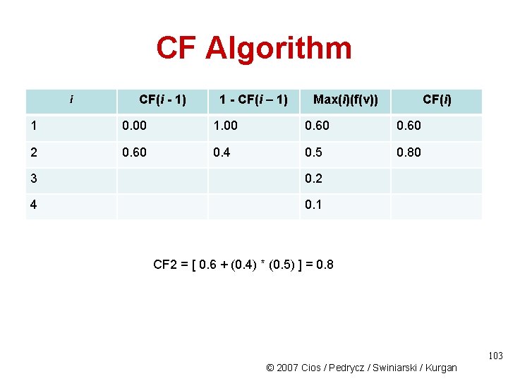
CF Algorithm i CF(i - 1) 1 - CF(i – 1) Max(i)(f(v)) CF(i) 1 0. 00 1. 00 0. 60 2 0. 60 0. 4 0. 5 0. 80 3 0. 2 4 0. 1 CF 2 = [ 0. 6 + (0. 4) * (0. 5) ] = 0. 8 103 © 2007 Cios / Pedrycz / Swiniarski / Kurgan

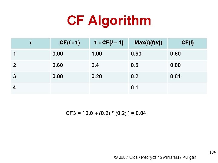
CF Algorithm i CF(i - 1) 1 - CF(i – 1) Max(i)(f(v)) CF(i) 1 0. 00 1. 00 0. 60 2 0. 60 0. 4 0. 5 0. 80 3 0. 80 0. 2 0. 84 4 0. 1 CF 3 = [ 0. 8 + (0. 2) * (0. 2) ] = 0. 84 104 © 2007 Cios / Pedrycz / Swiniarski / Kurgan

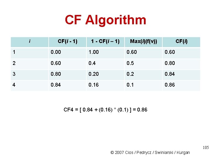
CF Algorithm i CF(i - 1) 1 - CF(i – 1) Max(i)(f(v)) CF(i) 1 0. 00 1. 00 0. 60 2 0. 60 0. 4 0. 5 0. 80 3 0. 80 0. 2 0. 84 4 0. 84 0. 16 0. 1 0. 86 CF 4 = [ 0. 84 + (0. 16) * (0. 1) ] = 0. 86 105 © 2007 Cios / Pedrycz / Swiniarski / Kurgan

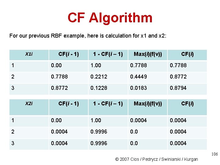
CF Algorithm For our previous RBF example, here is calculation for x 1 and x 2: X 1 i CF(i - 1) 1 - CF(i – 1) Max(i)(f(v)) CF(i) 1 0. 00 1. 00 0. 7788 2 0. 7788 0. 2212 0. 4449 0. 8772 3 0. 8772 0. 1228 0. 0183 0. 8794 X 2 i CF(i - 1) 1 - CF(i – 1) Max(i)(f(v)) CF(i) 1 0. 00 1. 00 0. 0004 2 0. 0004 0. 9996 0. 0004 3 0. 0004 0. 9996 0. 0004 106 © 2007 Cios / Pedrycz / Swiniarski / Kurgan

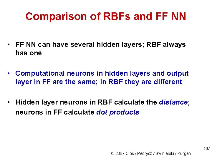
Comparison of RBFs and FF NN • FF NN can have several hidden layers; RBF always has one • Computational neurons in hidden layers and output layer in FF are the same; in RBF they are different • Hidden layer neurons in RBF calculate the distance; neurons in FF calculate dot products 107 © 2007 Cios / Pedrycz / Swiniarski / Kurgan

RBFs in Knowledge Discovery To overcome the problem of “black box” characteristic of NN, and to find a way to interpret weights and connections of an RBF network we can use: 1. Rule-based indirect interpretation of the RBF network 2. Fuzzy context-based RBF network 108 © 2007 Cios / Pedrycz / Swiniarski / Kurgan

Rule-Based Interpretation of RBF network is “equivalent” to a system of fuzzy production rules, i. e. , the RBF data model corresponds to a set of fuzzy rules (model) describing the same data. By using the correspondence the results can be interpreted and easily understood by humans. 109 © 2007 Cios / Pedrycz / Swiniarski / Kurgan

Approximation of training data via basis functions Фi and fuzzy sets Ai. 110 © 2007 Cios / Pedrycz / Swiniarski / Kurgan

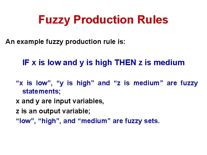
Fuzzy Production Rules An example fuzzy production rule is: IF x is low and y is high THEN z is medium “x is low”, “y is high” and “z is medium” are fuzzy statements; x and y are input variables, z is an output variable; “low”, “high”, and “medium” are fuzzy sets.

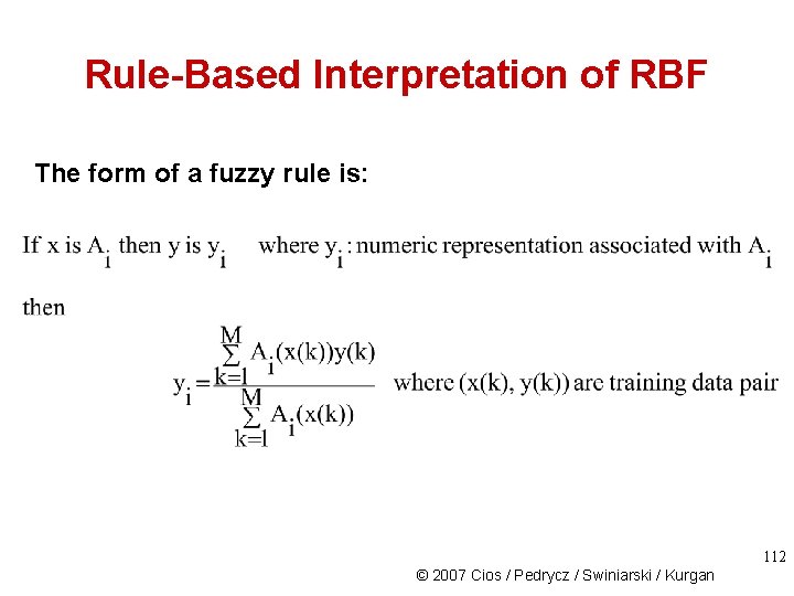
Rule-Based Interpretation of RBF The form of a fuzzy rule is: 112 © 2007 Cios / Pedrycz / Swiniarski / Kurgan

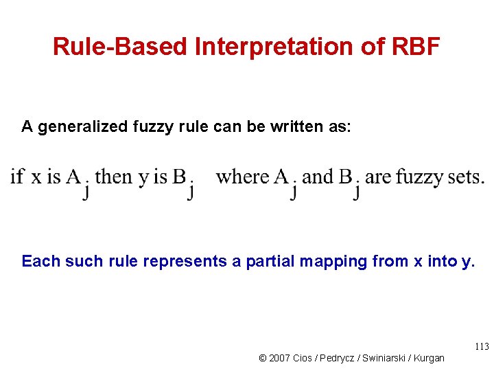
Rule-Based Interpretation of RBF A generalized fuzzy rule can be written as: Each such rule represents a partial mapping from x into y. 113 © 2007 Cios / Pedrycz / Swiniarski / Kurgan

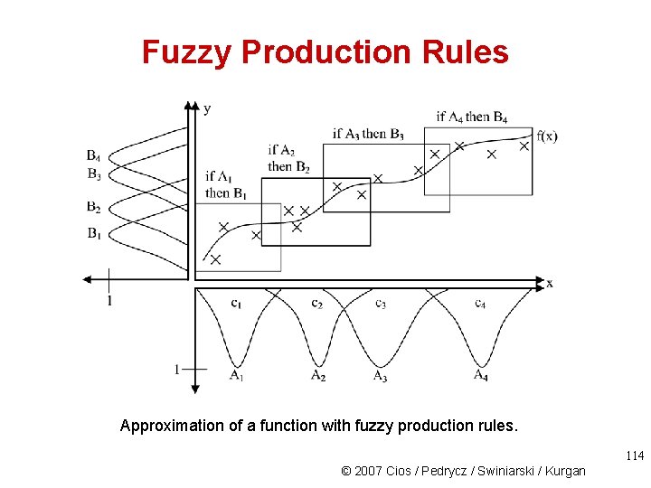
Fuzzy Production Rules Approximation of a function with fuzzy production rules. 114 © 2007 Cios / Pedrycz / Swiniarski / Kurgan

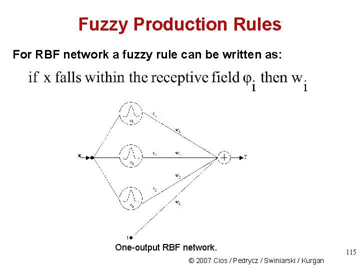
Fuzzy Production Rules For RBF network a fuzzy rule can be written as: One-output RBF network. © 2007 Cios / Pedrycz / Swiniarski / Kurgan 115

Fuzzy production rules system. 116 © 2007 Cios / Pedrycz / Swiniarski / Kurgan

RBF in Knowledge Discovery Fuzzy context-based RBF network – Fuzzy contexts, aka data mining windows, are used to select only pertinent records from a DB (Only records whose fields match a fuzzy context OUTPUT to a non-zero degree are retrieved) – As a result the selected input data are clustered 117 © 2007 Cios / Pedrycz / Swiniarski / Kurgan

Fuzzy context and its data windowing effect on the original training set 118 © 2007 Cios / Pedrycz / Swiniarski / Kurgan

Fuzzy Context-Based RBF Network For each context i we put pertinent data into ci clusters. This means that for p contexts, we end up with c 1, c 2, … cp clusters. The collection of these clusters defines the hidden layer of the RBF network. The outputs of the neurons of this layer are then linearly combined by the output-layer neuron(s). 119 © 2007 Cios / Pedrycz / Swiniarski / Kurgan

Fuzzy Context-Based RBF Network One advantage of using the fuzzy context is shortening of training time, which can be substantial for large databases. More importantly, the network can be directly interpreted as collection of IF…THEN…rules. 120 © 2007 Cios / Pedrycz / Swiniarski / Kurgan

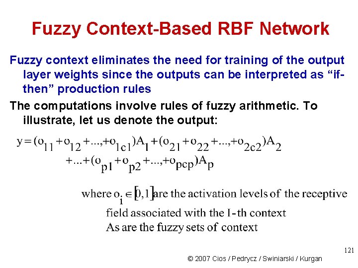
Fuzzy Context-Based RBF Network Fuzzy context eliminates the need for training of the output layer weights since the outputs can be interpreted as “ifthen” production rules The computations involve rules of fuzzy arithmetic. To illustrate, let us denote the output: 121 © 2007 Cios / Pedrycz / Swiniarski / Kurgan

Fuzzy sets of context. 122 © 2007 Cios / Pedrycz / Swiniarski / Kurgan

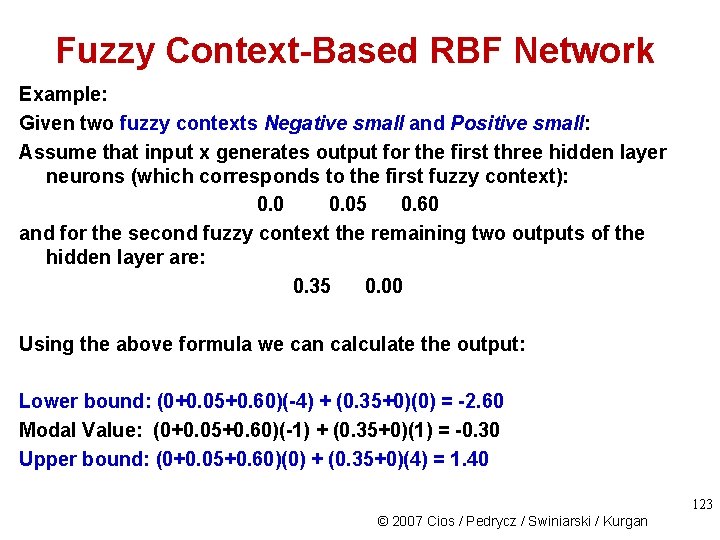
Fuzzy Context-Based RBF Network Example: Given two fuzzy contexts Negative small and Positive small: Assume that input x generates output for the first three hidden layer neurons (which corresponds to the first fuzzy context): 0. 05 0. 60 and for the second fuzzy context the remaining two outputs of the hidden layer are: 0. 35 0. 00 Using the above formula we can calculate the output: Lower bound: (0+0. 05+0. 60)(-4) + (0. 35+0)(0) = -2. 60 Modal Value: (0+0. 05+0. 60)(-1) + (0. 35+0)(1) = -0. 30 Upper bound: (0+0. 05+0. 60)(0) + (0. 35+0)(4) = 1. 40 123 © 2007 Cios / Pedrycz / Swiniarski / Kurgan

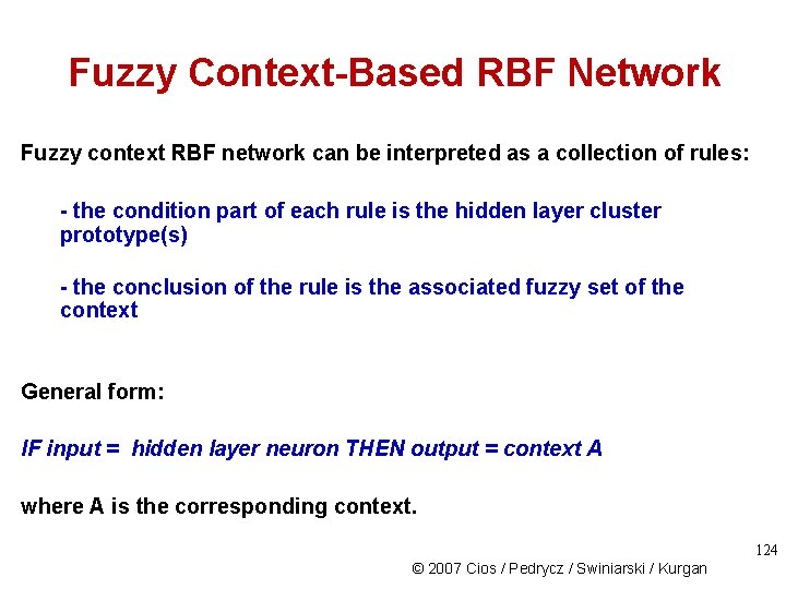
Fuzzy Context-Based RBF Network Fuzzy context RBF network can be interpreted as a collection of rules: - the condition part of each rule is the hidden layer cluster prototype(s) - the conclusion of the rule is the associated fuzzy set of the context General form: IF input = hidden layer neuron THEN output = context A where A is the corresponding context. 124 © 2007 Cios / Pedrycz / Swiniarski / Kurgan

References Broomhead, D. S. , and Lowe, D. 1988. Multivariable functional interpolation and adaptive networks. Complex Systems, 2: 321 -355. Cios, K. J. , and Pedrycz , W. 1997. Neuro-fuzzy systems. In: Handbook on Neural Computation. Oxford University Press, D 1. 1 - D 1. 8 Cios, K. J. , Pedrycz, W. , and Swiniarski R. 1998. Data Mining Methods for Knowledge Discovery. Kluwer Hebb, D. O. 1949. The Organization of Behavior. Wiley Kecman, V. , and Pfeiffer, B. M. 1994. Exploiting the structural equivalence of learning fuzzy systems and radial basis function neural networks. In: Proceedings of EUFIT’ 94, Aachen. 1: 58 -66 Kecman, V. 2001. Learning and Soft Computing. MIT Press 125 © 2007 Cios / Pedrycz / Swiniarski / Kurgan

References Mc. Culloch, W. S. , and Pitts, W. H. 1943. A logical calculus of the ideas immanent in nervous activity. Bulletin of Mathematics and Biophysics, 5: 115 -133 Pedrycz, W. 1998. Conditional fuzzy clustering in the design of radial basis function neural networks. IEEE Transactions on Neural Networks, 9(4): 601 -612 Pedrycz, W. , and Vasilakos, A. V. 1999. Linguistic models and linguistic modeling. IEEE Transactions on Systems, Man, and Cybernetics, Part C, 29(6): 745 -757 Poggio, F. 1994. Regularization theory, radial basis functions and networks. In: From Statistics to Neural Networks: Theory and Pattern Recognition Applications, NATO ASI Series, 136: 83 -104 Swiercz, W. , Cios, K. J. , Staley, K. , Kurgan, L. , Accurso, F. , and Sagel S. 2006. New synaptic plasticity rule for networks of spiking neurons, IEEE Transactions on Neural Networks, 17(1): 94 -105 Wedding, D. K. II, and Cios, K. J. 1998. Certainty factors versus Parzen windows as reliability measures in RBF networks. Neurocomputing, 19(1 -3): 151 -165 126 © 2007 Cios / Pedrycz / Swiniarski / Kurgan