Chapter 13 Simple Linear Regression Analysis Mc GrawHillIrwin

Chapter 13 Simple Linear Regression Analysis Mc. Graw-Hill/Irwin Copyright © 2009 by The Mc. Graw-Hill Companies, Inc. All Rights Reserved.

Simple Linear Regression 13. 1 The Simple Linear Regression Model and the Least Square Point Estimates 13. 2 Model Assumptions and the Standard Error 13. 3 Testing the Significance of Slope and y-Intercept 13. 4 Confidence and Prediction Intervals 13 -2

Simple Linear Regression Continued 13. 5 Simple Coefficients of Determination and Correlation 13. 6 Testing the Significance of the Population Correlation Coefficient (Optional) 13. 7 An F Test for the Model 13. 8 Residual Analysis (Optional) 13. 9 Some Shortcut Formulas (Optional) 13 -3

The Simple Linear Regression Model and the Least Squares Point Estimates • The dependent (or response) variable is the variable we wish to understand or predict • The independent (or predictor) variable is the variable we will use to understand or predict the dependent variable • Regression analysis is a statistical technique that uses observed data to relate the dependent variable to one or more independent variables 13 -4

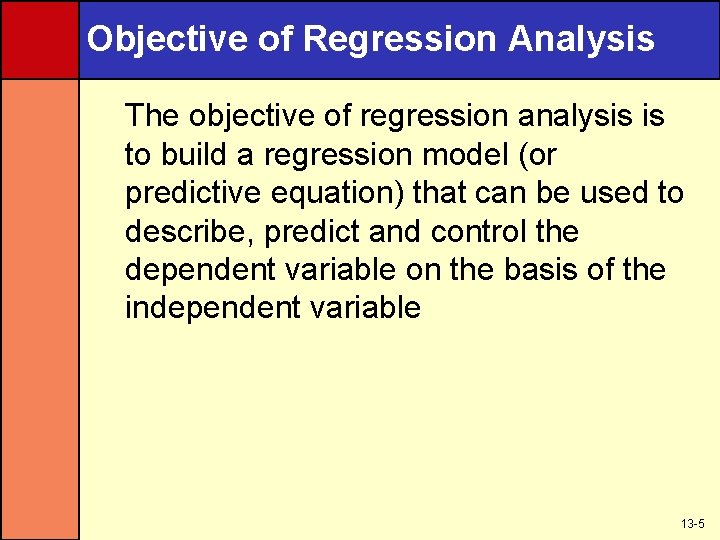
Objective of Regression Analysis The objective of regression analysis is to build a regression model (or predictive equation) that can be used to describe, predict and control the dependent variable on the basis of the independent variable 13 -5

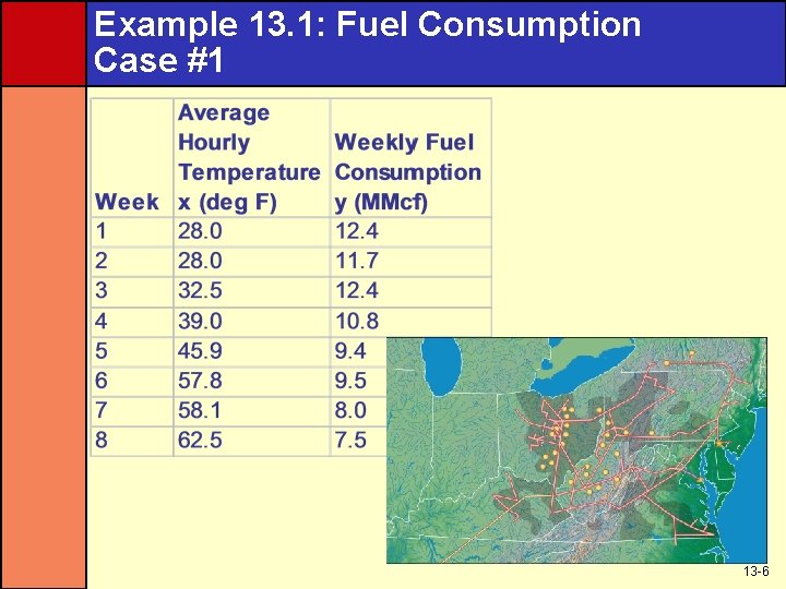
Example 13. 1: Fuel Consumption Case #1 13 -6

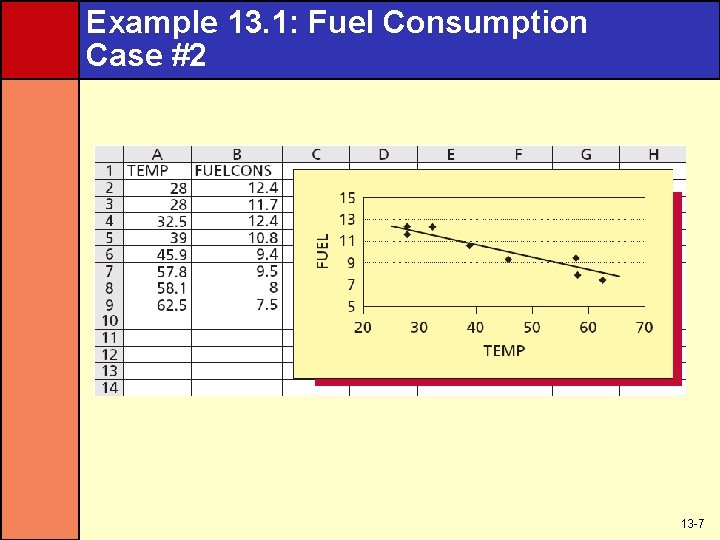
Example 13. 1: Fuel Consumption Case #2 13 -7

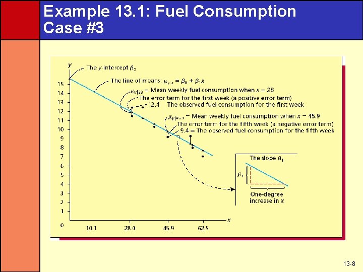
Example 13. 1: Fuel Consumption Case #3 13 -8

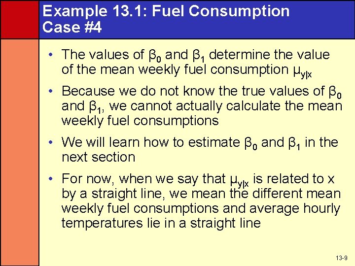
Example 13. 1: Fuel Consumption Case #4 • The values of β 0 and β 1 determine the value of the mean weekly fuel consumption μy|x • Because we do not know the true values of β 0 and β 1, we cannot actually calculate the mean weekly fuel consumptions • We will learn how to estimate β 0 and β 1 in the next section • For now, when we say that μy|x is related to x by a straight line, we mean the different mean weekly fuel consumptions and average hourly temperatures lie in a straight line 13 -9

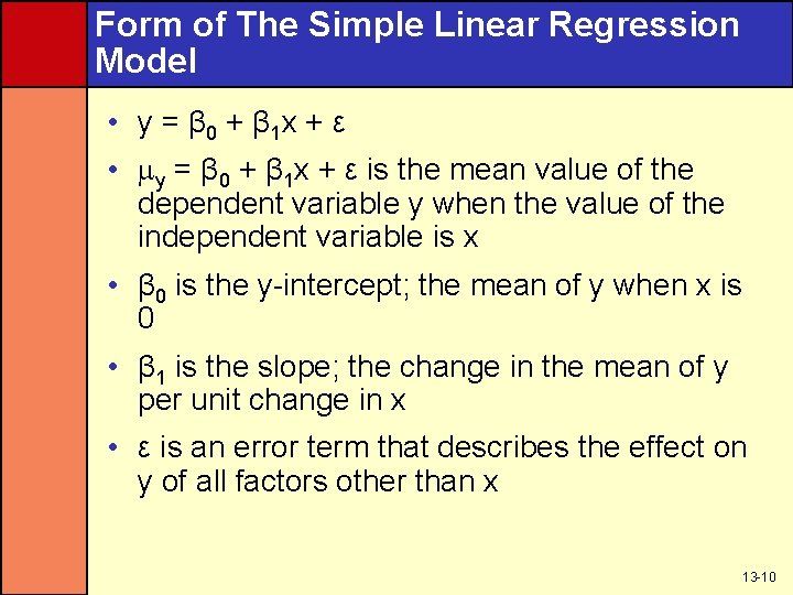
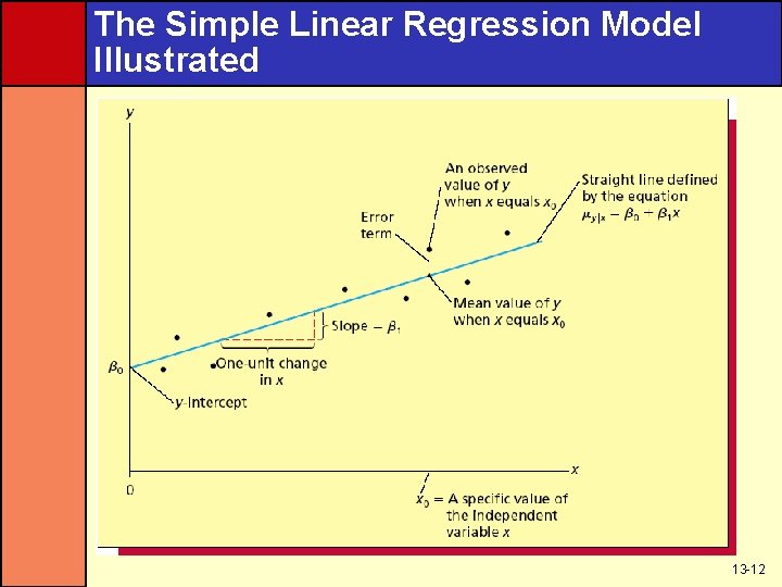
Form of The Simple Linear Regression Model • y = β 0 + β 1 x + ε • y = β 0 + β 1 x + ε is the mean value of the dependent variable y when the value of the independent variable is x • β 0 is the y-intercept; the mean of y when x is 0 • β 1 is the slope; the change in the mean of y per unit change in x • ε is an error term that describes the effect on y of all factors other than x 13 -10

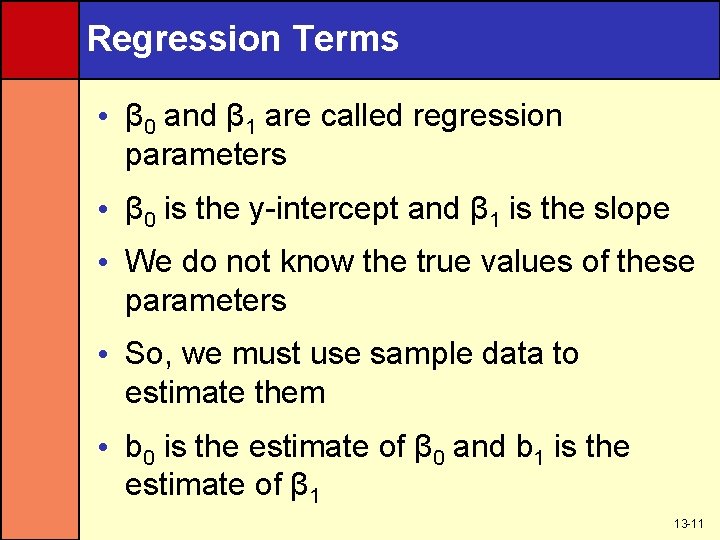
Regression Terms • β 0 and β 1 are called regression parameters • β 0 is the y-intercept and β 1 is the slope • We do not know the true values of these parameters • So, we must use sample data to estimate them • b 0 is the estimate of β 0 and b 1 is the estimate of β 1 13 -11

The Simple Linear Regression Model Illustrated 13 -12

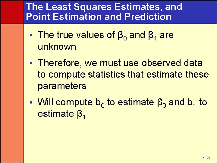
The Least Squares Estimates, and Point Estimation and Prediction • The true values of β 0 and β 1 are unknown • Therefore, we must use observed data to compute statistics that estimate these parameters • Will compute b 0 to estimate β 0 and b 1 to estimate β 1 13 -13

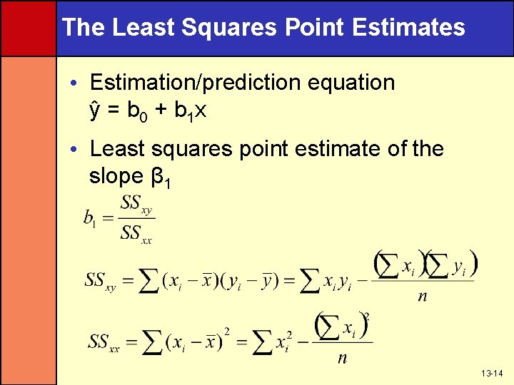
The Least Squares Point Estimates • Estimation/prediction equation y = b 0 + b 1 x • Least squares point estimate of the slope β 1 13 -14

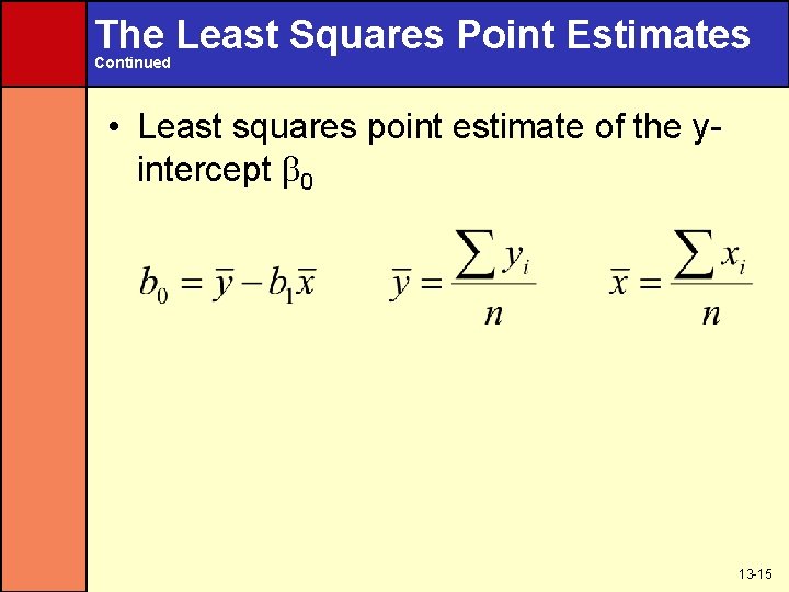
The Least Squares Point Estimates Continued • Least squares point estimate of the yintercept 0 13 -15

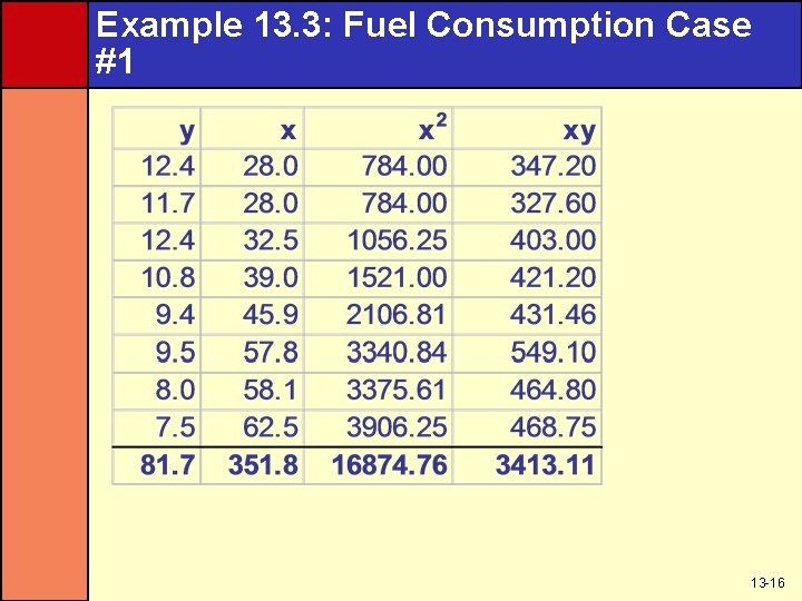
Example 13. 3: Fuel Consumption Case #1 13 -16

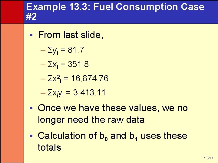
Example 13. 3: Fuel Consumption Case #2 • From last slide, – Σyi = 81. 7 – Σxi = 351. 8 – Σx 2 i = 16, 874. 76 – Σxiyi = 3, 413. 11 • Once we have these values, we no longer need the raw data • Calculation of b 0 and b 1 uses these totals 13 -17

Example 13. 3: Fuel Consumption Case #3 (Slope b 1) 13 -18

Example 13. 3: Fuel Consumption Case #4 (y-Intercept b 0) 13 -19

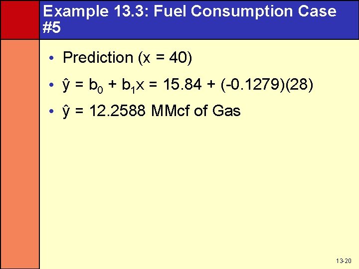
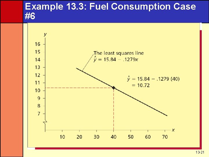
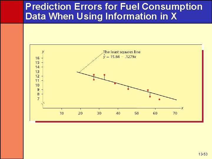
Example 13. 3: Fuel Consumption Case #5 • Prediction (x = 40) • y = b 0 + b 1 x = 15. 84 + (-0. 1279)(28) • y = 12. 2588 MMcf of Gas 13 -20

Example 13. 3: Fuel Consumption Case #6 13 -21

Example 13. 3: The Danger of Extrapolation Outside The Experimental Region 13 -22

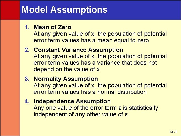
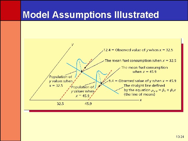
Model Assumptions 1. Mean of Zero At any given value of x, the population of potential error term values has a mean equal to zero 2. Constant Variance Assumption At any given value of x, the population of potential error term values has a variance that does not depend on the value of x 3. Normality Assumption At any given value of x, the population of potential error term values has a normal distribution 4. Independence Assumption Any one value of the error term ε is statistically independent of any other value of ε 13 -23

Model Assumptions Illustrated 13 -24

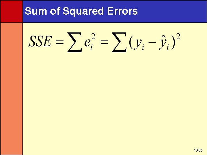
Sum of Squared Errors 13 -25

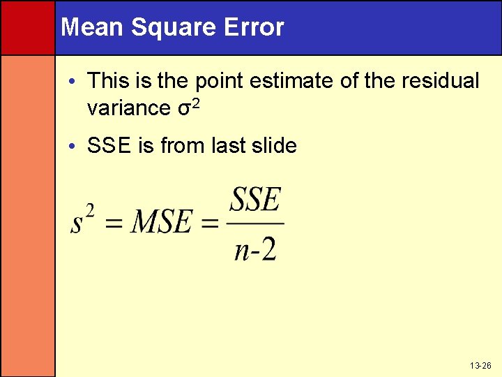
Mean Square Error • This is the point estimate of the residual variance σ2 • SSE is from last slide 13 -26

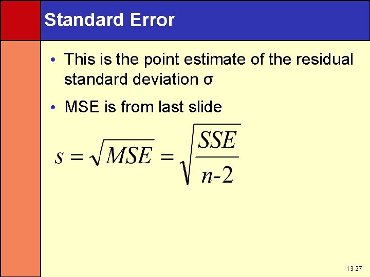
Standard Error • This is the point estimate of the residual standard deviation σ • MSE is from last slide 13 -27

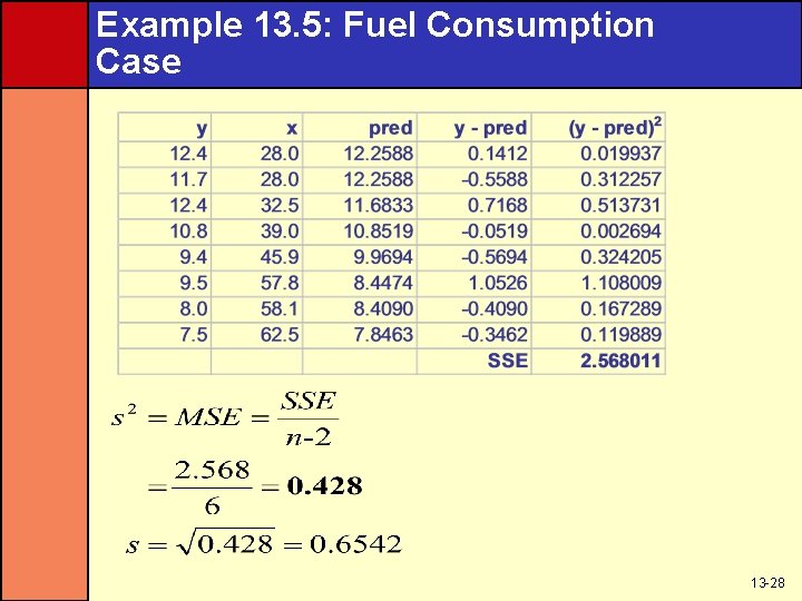
Example 13. 5: Fuel Consumption Case 13 -28

Testing the Significance of the Slope • A regression model is not likely to be useful unless there is a significant relationship between x and y • To test significance, we use the null hypothesis: H 0: β 1 = 0 • Versus the alternative hypothesis: H a: β 1 ≠ 0 13 -29

Testing the Significance of the Slope #2 If the regression assumptions hold, we can reject H 0: 1 = 0 at the level of significance (probability of Type I error equal to ) if and only if the appropriate rejection point condition holds or, equivalently, if the corresponding pvalue is less than 13 -30

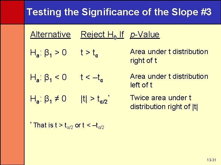
Testing the Significance of the Slope #3 Alternative Reject H 0 If p-Value H a: β 1 > 0 t > tα Area under t distribution right of t H a: β 1 < 0 t < –tα Area under t distribution left of t H a: β 1 ≠ 0 |t| > tα/2* Twice area under t distribution right of |t| * That is t > tα/2 or t < –tα/2 13 -31

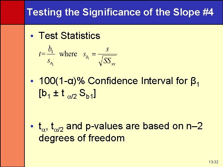
Testing the Significance of the Slope #4 • Test Statistics • 100(1 -α)% Confidence Interval for β 1 [b 1 ± t /2 Sb 1] • t , t /2 and p-values are based on n– 2 degrees of freedom 13 -32

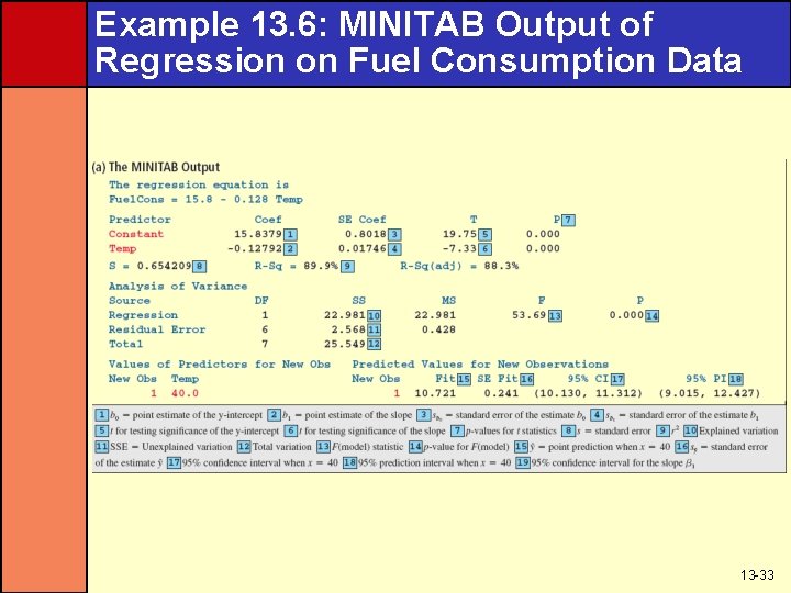
Example 13. 6: MINITAB Output of Regression on Fuel Consumption Data 13 -33

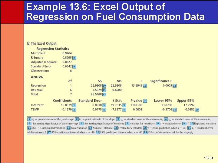
Example 13. 6: Excel Output of Regression on Fuel Consumption Data 13 -34

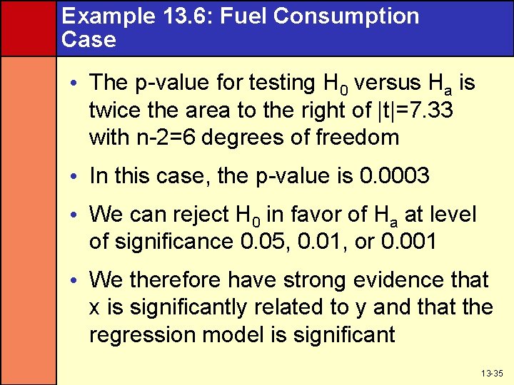
Example 13. 6: Fuel Consumption Case • The p-value for testing H 0 versus Ha is twice the area to the right of |t|=7. 33 with n-2=6 degrees of freedom • In this case, the p-value is 0. 0003 • We can reject H 0 in favor of Ha at level of significance 0. 05, 0. 01, or 0. 001 • We therefore have strong evidence that x is significantly related to y and that the regression model is significant 13 -35

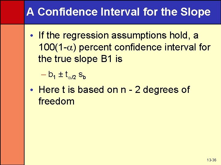
A Confidence Interval for the Slope • If the regression assumptions hold, a 100(1 - ) percent confidence interval for the true slope B 1 is – b 1 ± t /2 sb • Here t is based on n - 2 degrees of freedom 13 -36

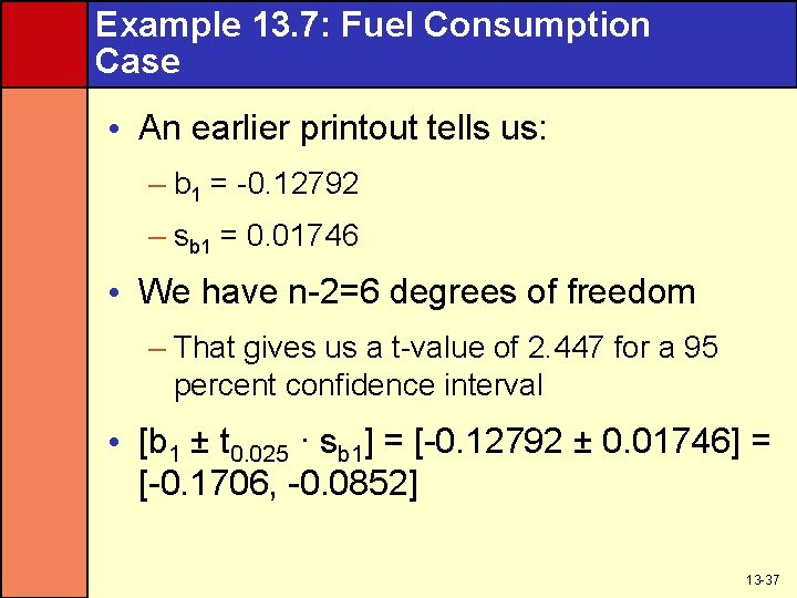
Example 13. 7: Fuel Consumption Case • An earlier printout tells us: – b 1 = -0. 12792 – sb 1 = 0. 01746 • We have n-2=6 degrees of freedom – That gives us a t-value of 2. 447 for a 95 percent confidence interval • [b 1 ± t 0. 025 · sb 1] = [-0. 12792 ± 0. 01746] = [-0. 1706, -0. 0852] 13 -37

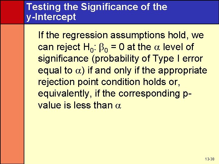
Testing the Significance of the y-Intercept If the regression assumptions hold, we can reject H 0: 0 = 0 at the level of significance (probability of Type I error equal to ) if and only if the appropriate rejection point condition holds or, equivalently, if the corresponding pvalue is less than 13 -38

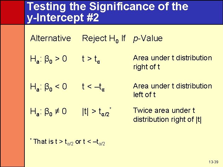
Testing the Significance of the y-Intercept #2 Alternative Reject H 0 If p-Value H a: β 0 > 0 t > tα Area under t distribution right of t H a: β 0 < 0 t < –tα Area under t distribution left of t H a: β 0 ≠ 0 |t| > tα/2* Twice area under t distribution right of |t| * That is t > tα/2 or t < –tα/2 13 -39

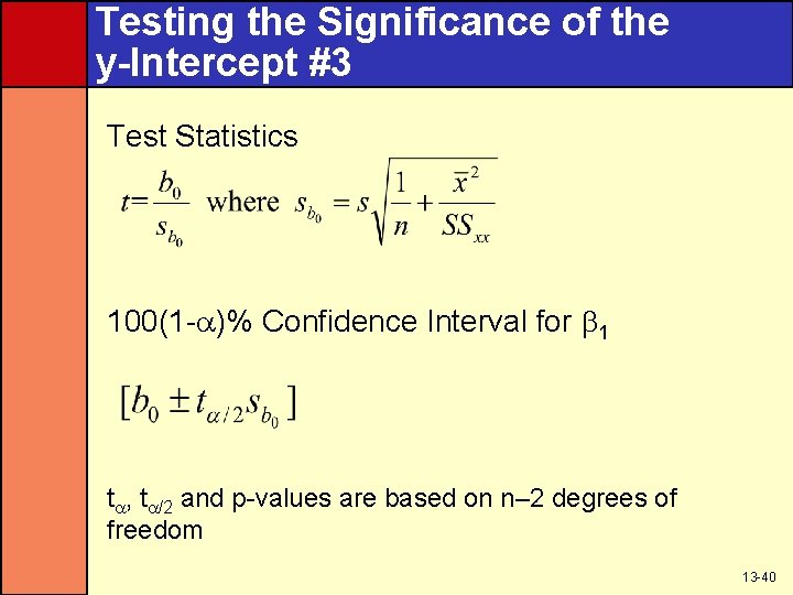
Testing the Significance of the y-Intercept #3 Test Statistics 100(1 - )% Confidence Interval for 1 t , t /2 and p-values are based on n– 2 degrees of freedom 13 -40

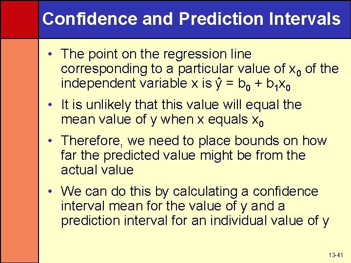
Confidence and Prediction Intervals • The point on the regression line corresponding to a particular value of x 0 of the independent variable x is y = b 0 + b 1 x 0 • It is unlikely that this value will equal the mean value of y when x equals x 0 • Therefore, we need to place bounds on how far the predicted value might be from the actual value • We can do this by calculating a confidence interval mean for the value of y and a prediction interval for an individual value of y 13 -41

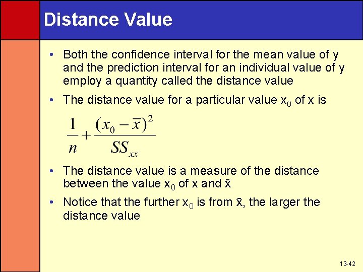
Distance Value • Both the confidence interval for the mean value of y and the prediction interval for an individual value of y employ a quantity called the distance value • The distance value for a particular value x 0 of x is • The distance value is a measure of the distance between the value x 0 of x and x • Notice that the further x 0 is from x, the larger the distance value 13 -42

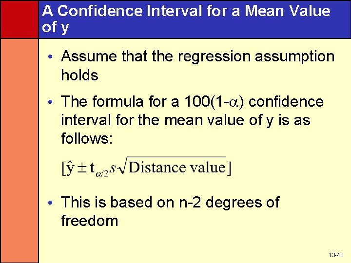
A Confidence Interval for a Mean Value of y • Assume that the regression assumption holds • The formula for a 100(1 - ) confidence interval for the mean value of y is as follows: • This is based on n-2 degrees of freedom 13 -43

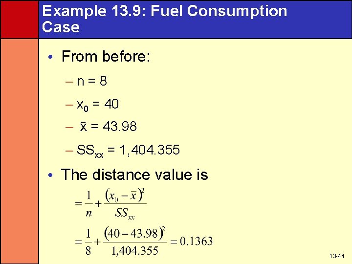
Example 13. 9: Fuel Consumption Case • From before: –n=8 – x 0 = 40 – x = 43. 98 – SSxx = 1, 404. 355 • The distance value is 13 -44

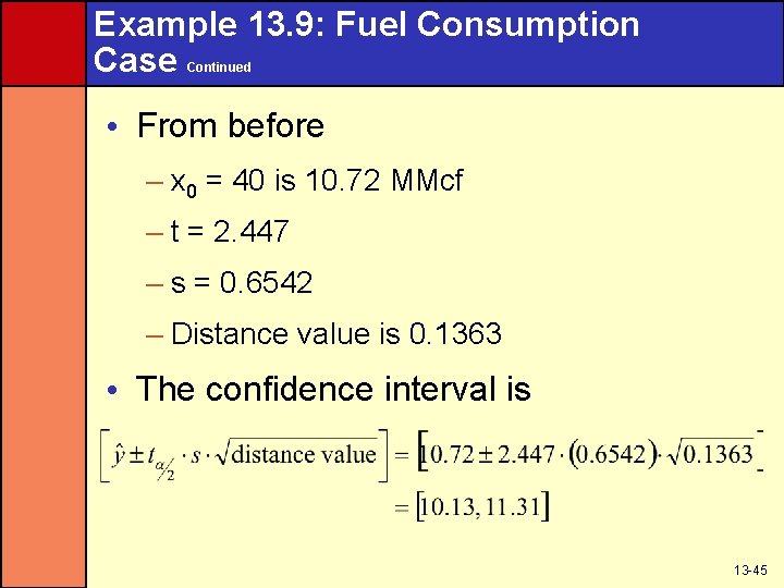
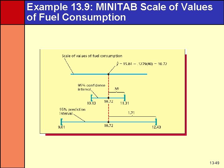
Example 13. 9: Fuel Consumption Case Continued • From before – x 0 = 40 is 10. 72 MMcf – t = 2. 447 – s = 0. 6542 – Distance value is 0. 1363 • The confidence interval is 13 -45

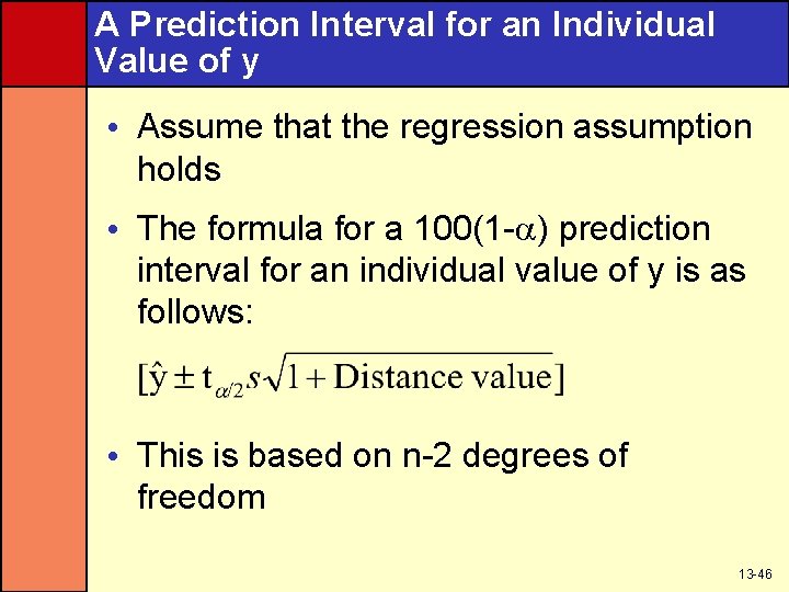
A Prediction Interval for an Individual Value of y • Assume that the regression assumption holds • The formula for a 100(1 - ) prediction interval for an individual value of y is as follows: • This is based on n-2 degrees of freedom 13 -46

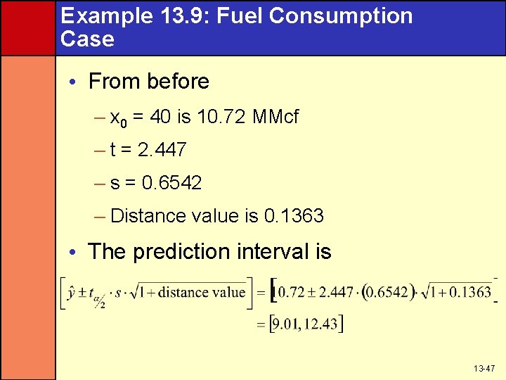
Example 13. 9: Fuel Consumption Case • From before – x 0 = 40 is 10. 72 MMcf – t = 2. 447 – s = 0. 6542 – Distance value is 0. 1363 • The prediction interval is 13 -47

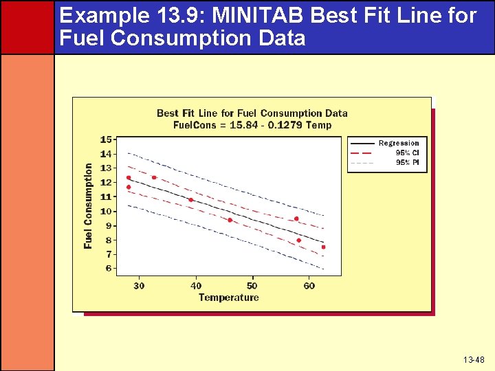
Example 13. 9: MINITAB Best Fit Line for Fuel Consumption Data 13 -48

Example 13. 9: MINITAB Scale of Values of Fuel Consumption 13 -49

Which to Use? • The prediction interval is useful if it is important to predict an individual value of the dependent variable • A confidence interval is useful if it is important to estimate the mean value • The prediction interval will always be wider than the confidence interval 13 -50

The Simple Coefficient of Determination and Correlation • How useful is a particular regression model? • One measure of usefulness is the simple coefficient of determination • It is represented by the symbol r 2 13 -51

Prediction Errors for Fuel Consumption Data When Not Using Information in X 13 -52

Prediction Errors for Fuel Consumption Data When Using Information in X 13 -53

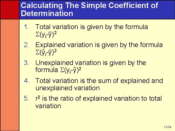
Calculating The Simple Coefficient of Determination 1. Total variation is given by the formula (yi-y )2 2. Explained variation is given by the formula (y i-y )2 3. Unexplained variation is given by the formula (yi-y )2 4. Total variation is the sum of explained and unexplained variation 5. r 2 is the ratio of explained variation to total variation 13 -54

What Does r 2 Mean? The coefficient of determination, r 2, is the proportion of the total variation in the n observed values of the dependent variable that is explained by the simple linear regression model 13 -55

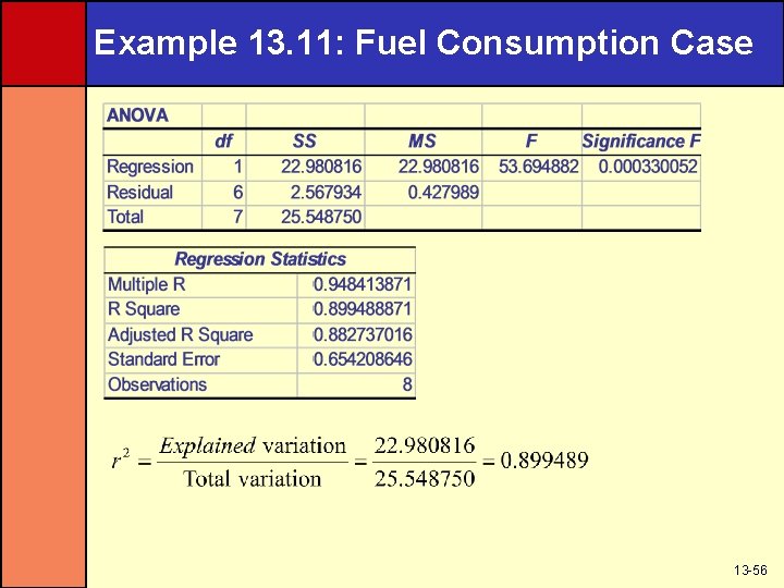
Example 13. 11: Fuel Consumption Case 13 -56

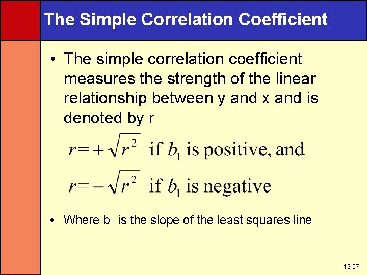
The Simple Correlation Coefficient • The simple correlation coefficient measures the strength of the linear relationship between y and x and is denoted by r • Where b 1 is the slope of the least squares line 13 -57

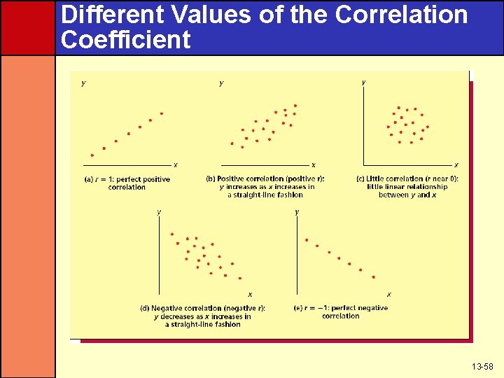
Different Values of the Correlation Coefficient 13 -58

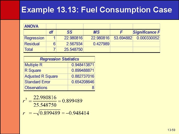
Example 13. 13: Fuel Consumption Case 13 -59

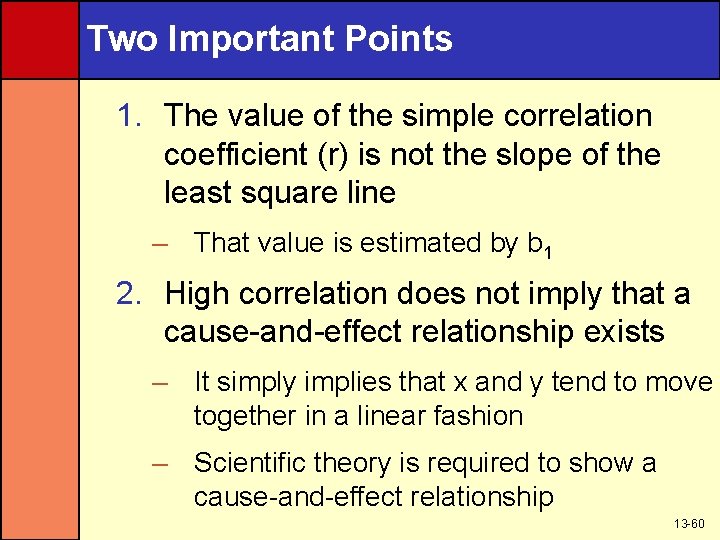
Two Important Points 1. The value of the simple correlation coefficient (r) is not the slope of the least square line – That value is estimated by b 1 2. High correlation does not imply that a cause-and-effect relationship exists – It simply implies that x and y tend to move together in a linear fashion – Scientific theory is required to show a cause-and-effect relationship 13 -60

Testing the Significance of the Population Correlation Coefficient • The simple correlation coefficient (r) measures the linear relationship between the observed values of x and y from the sample • The population correlation coefficient (ρ) measures the linear relationship between all possible combinations of observed values of x and y • r is an estimate of ρ 13 -61

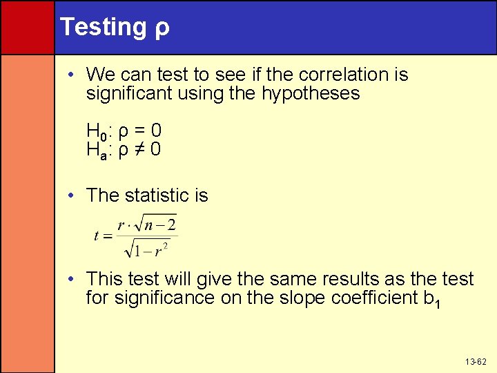
Testing ρ • We can test to see if the correlation is significant using the hypotheses H 0: ρ = 0 H a: ρ ≠ 0 • The statistic is • This test will give the same results as the test for significance on the slope coefficient b 1 13 -62

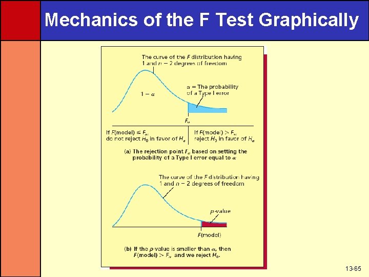
An F Test for Model • For simple regression, this is another way to test the null hypothesis H 0: β 1 = 0 • This is the only test we will use for multiple regression • The F tests the significance of the overall regression relationship between x and y 13 -63

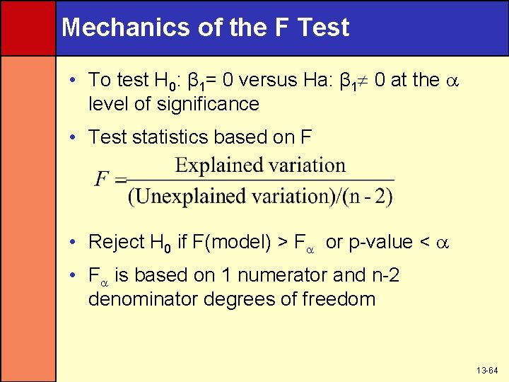
Mechanics of the F Test • To test H 0: β 1= 0 versus Ha: β 1 0 at the level of significance • Test statistics based on F • Reject H 0 if F(model) > F or p-value < • F is based on 1 numerator and n-2 denominator degrees of freedom 13 -64

Mechanics of the F Test Graphically 13 -65

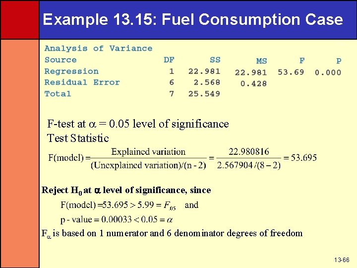
Example 13. 15: Fuel Consumption Case F-test at = 0. 05 level of significance Test Statistic Reject H 0 at level of significance, since F is based on 1 numerator and 6 denominator degrees of freedom 13 -66

Residual Analysis #1 • Checks of regression assumptions are performed by analyzing the regression residuals • Residuals (e) are defined as the difference between the observed value of y and the predicted value of y, e = y - y • Note that e is the point estimate of ε • If the regression assumptions are valid, the population of potential error terms will be normally distributed with a mean of zero and a variance σ2 • Furthermore, the different error terms will be statistically independent 13 -67

Residual Analysis #2 • The residuals should look like they have been randomly and independently selected from normally distributed populations having mean zero and variance σ2 • With any real data, assumptions will not hold exactly • Mild departures do not affect our ability to make statistical inferences • In checking assumptions, we are looking for pronounced departures from the assumptions • So, only require residuals to approximately fit the description above 13 -68

Residual Plots 1. Residuals versus independent variable 2. Residuals versus predicted y’s 3. Residuals in time order (if the response is a time series) 13 -69

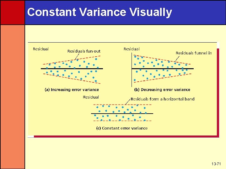
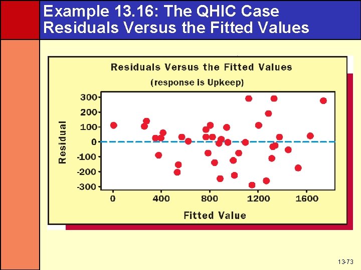
Constant Variance Assumptions • To check the validity of the constant variance assumption, examine residual plots against – The x values – The predicted y values – Time (when data is time series) • A pattern that fans out says the variance is increasing rather than staying constant • A pattern that funnels in says the variance is decreasing rather than staying constant • A pattern that is evenly spread within a band says the assumption has been met 13 -70

Constant Variance Visually 13 -71

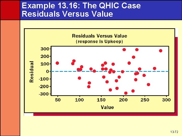
Example 13. 16: The QHIC Case Residuals Versus Value 13 -72

Example 13. 16: The QHIC Case Residuals Versus the Fitted Values 13 -73

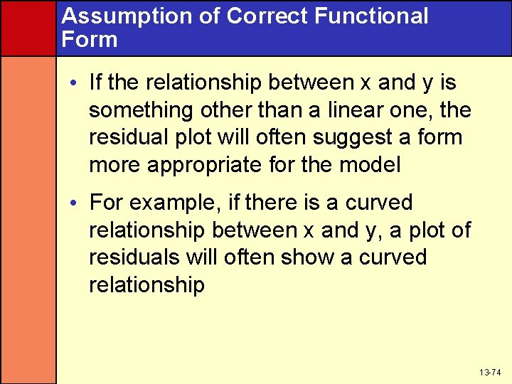
Assumption of Correct Functional Form • If the relationship between x and y is something other than a linear one, the residual plot will often suggest a form more appropriate for the model • For example, if there is a curved relationship between x and y, a plot of residuals will often show a curved relationship 13 -74

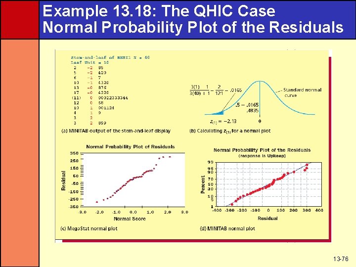
Normality Assumption • If the normality assumption holds, a histogram or stem-and-leaf display of residuals should look bell-shaped and symmetric • Another way to check is a normal plot of residuals – Order residuals from smallest to largest – Plot e(i) on vertical axis against z(i) • Z(i) is the point on the horizontal axis under the z curve so the area under this curve to the left is (3 i-1)/(3 n+1) • If the normality assumption holds, the plot should have a straight-line appearance 13 -75

Example 13. 18: The QHIC Case Normal Probability Plot of the Residuals 13 -76

Independence Assumption • Independence assumption is most likely to be violated when the data are time-series data – If the data is not time series, then it can be reordered without affecting the data – Changing the order would change the interdependence of the data • For time-series data, the time-ordered error terms can be autocorrelated – Positive autocorrelation is when a positive error term in time period i tends to be followed by another positive value in i+k – Negative autocorrelation is when a positive error term in time period i tends to be followed by a negative value in i+k • Either one will cause a cyclical error term over time 13 -77

Independence Assumption Visually Positive Autocorrelation 13 -78

Independence Assumption Visually Negative Autocorrelation 13 -79

Some Shortcut Formulas where 13 -80