Chapter 13 PROFIT MAXIMIZATION AND SUPPLY MICROECONOMIC THEORY

Chapter 13 PROFIT MAXIMIZATION AND SUPPLY MICROECONOMIC THEORY BASIC PRINCIPLES AND EXTENSIONS EIGHTH EDITION WALTER NICHOLSON Copyright © 2002 by South-Western, a division of Thomson Learning. All rights reserved.

The Nature of Firms • A firm is an association of individuals who have organized themselves for the purpose of turning inputs into outputs • Different individuals will provide different types of inputs – the nature of the contractual relationship between the providers of inputs to a firm may be quite complicated

Contractual Relationships • Some contracts between providers of inputs may be explicit – may specify hours, work details, or compensation • Other arrangements will be more implicit in nature – decision-making authority or sharing of tasks

Modeling Firms’ Behavior • Most economists treat the firm as a single decision-making unit – the decisions are made by a single dictatorial manager who rationally pursues some goal • profit-maximization

Profit Maximization • A profit-maximizing firm chooses both its inputs and its outputs with the sole goal of achieving maximum economic profits – seeks to maximize the difference between total revenue and total economic costs

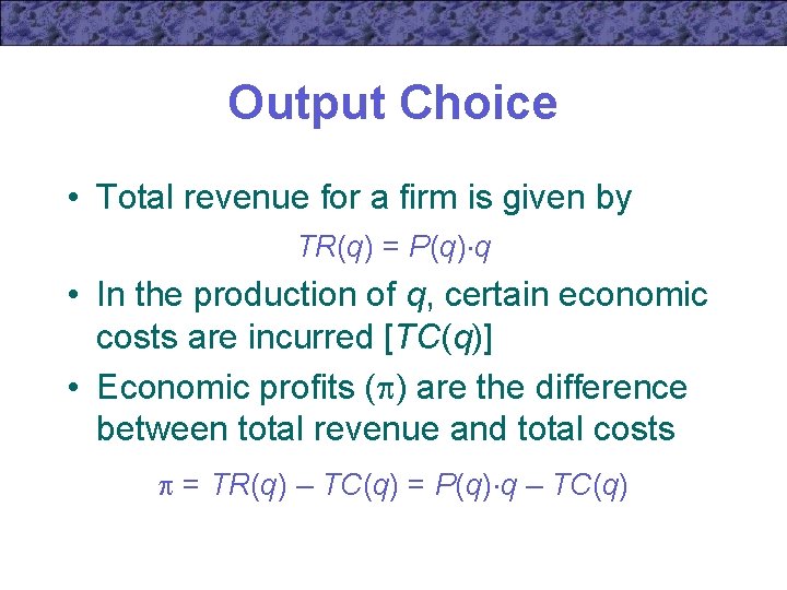
Output Choice • Total revenue for a firm is given by TR(q) = P(q) q • In the production of q, certain economic costs are incurred [TC(q)] • Economic profits ( ) are the difference between total revenue and total costs = TR(q) – TC(q) = P(q) q – TC(q)

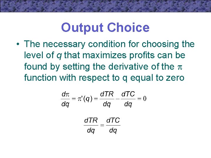
Output Choice • The necessary condition for choosing the level of q that maximizes profits can be found by setting the derivative of the function with respect to q equal to zero

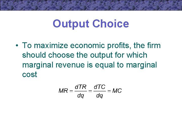
Output Choice • To maximize economic profits, the firm should choose the output for which marginal revenue is equal to marginal cost

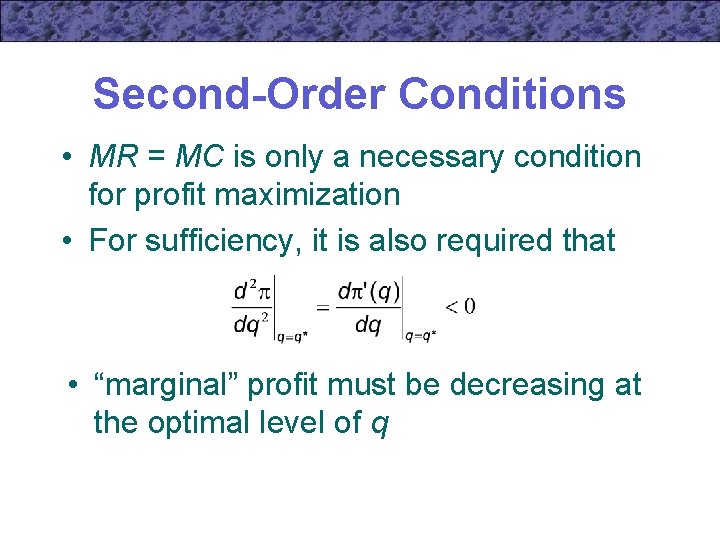
Second-Order Conditions • MR = MC is only a necessary condition for profit maximization • For sufficiency, it is also required that • “marginal” profit must be decreasing at the optimal level of q

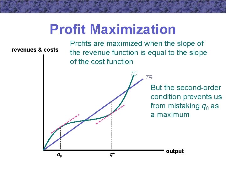
Profit Maximization revenues & costs Profits are maximized when the slope of the revenue function is equal to the slope of the cost function TC TR But the second-order condition prevents us from mistaking q 0 as a maximum q 0 q* output

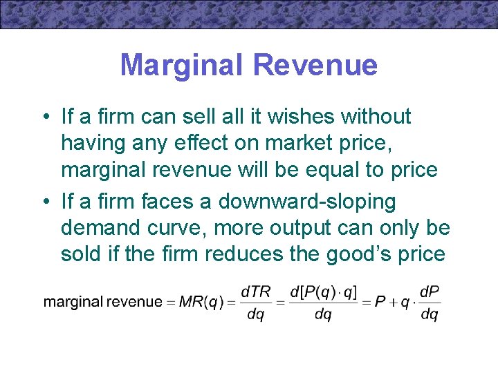
Marginal Revenue • If a firm can sell all it wishes without having any effect on market price, marginal revenue will be equal to price • If a firm faces a downward-sloping demand curve, more output can only be sold if the firm reduces the good’s price

Marginal Revenue • If a firm faces a downward-sloping demand curve, marginal revenue will be a function of output • If price falls as a firm increases output, marginal revenue will be less than price

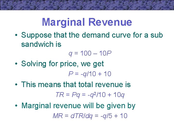
Marginal Revenue • Suppose that the demand curve for a sub sandwich is q = 100 – 10 P • Solving for price, we get P = -q/10 + 10 • This means that total revenue is TR = Pq = -q 2/10 + 10 q • Marginal revenue will be given by MR = d. TR/dq = -q/5 + 10

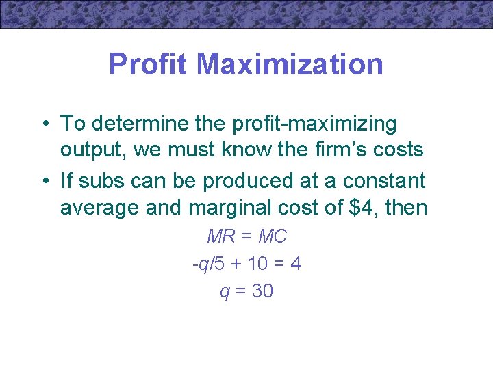
Profit Maximization • To determine the profit-maximizing output, we must know the firm’s costs • If subs can be produced at a constant average and marginal cost of $4, then MR = MC -q/5 + 10 = 4 q = 30

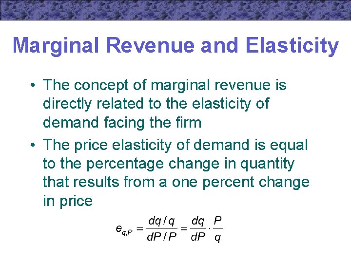
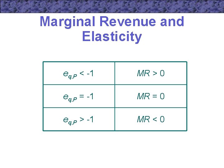
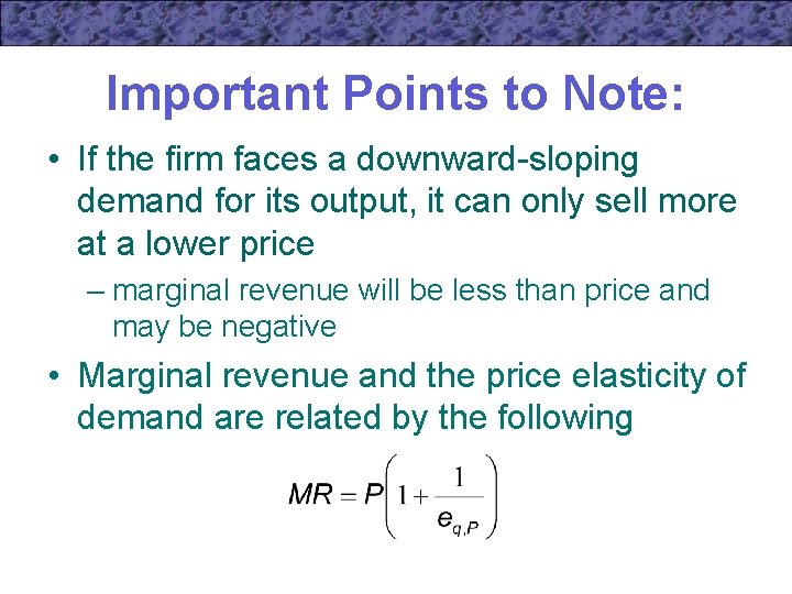
Marginal Revenue and Elasticity • The concept of marginal revenue is directly related to the elasticity of demand facing the firm • The price elasticity of demand is equal to the percentage change in quantity that results from a one percent change in price

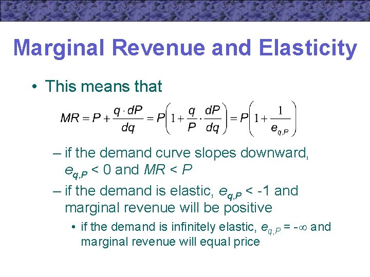
Marginal Revenue and Elasticity • This means that – if the demand curve slopes downward, eq, P < 0 and MR < P – if the demand is elastic, eq, P < -1 and marginal revenue will be positive • if the demand is infinitely elastic, eq, P = - and marginal revenue will equal price

Marginal Revenue and Elasticity eq, P < -1 MR > 0 eq, P = -1 MR = 0 eq, P > -1 MR < 0

Average Revenue Curve • If we assume that the firm must sell all its output at one price, we can think of the demand curve facing the firm as its average revenue curve – shows the revenue per unit yielded by alternative output choices

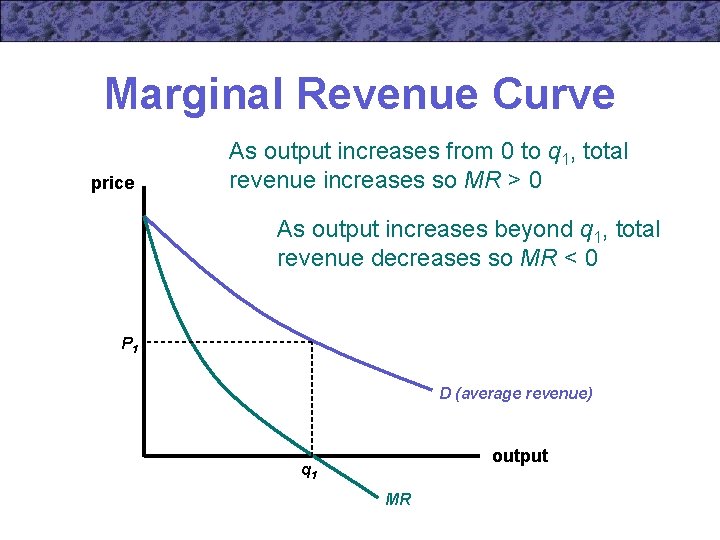
Marginal Revenue Curve • The marginal revenue curve shows the extra revenue provided by the last unit sold • In the case of a downward-sloping demand curve, the marginal revenue curve will lie below the demand curve

Marginal Revenue Curve price As output increases from 0 to q 1, total revenue increases so MR > 0 As output increases beyond q 1, total revenue decreases so MR < 0 P 1 D (average revenue) output q 1 MR

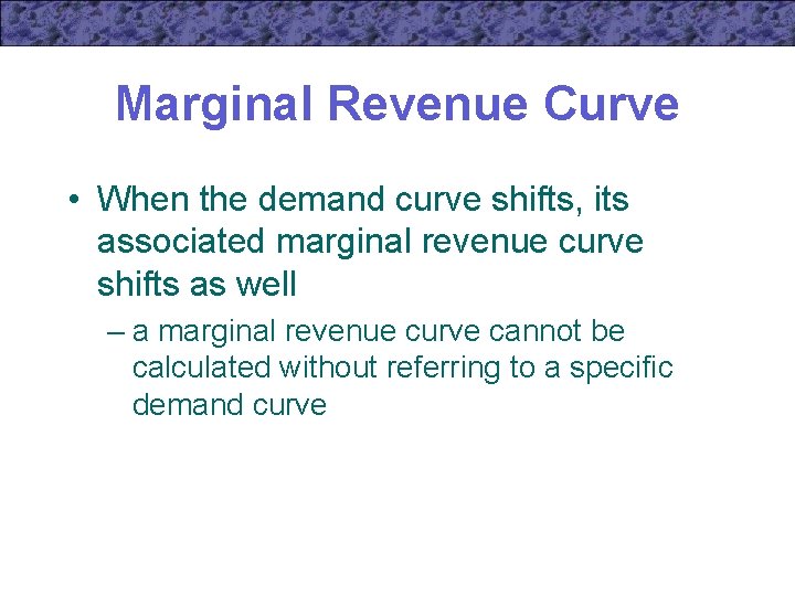
Marginal Revenue Curve • When the demand curve shifts, its associated marginal revenue curve shifts as well – a marginal revenue curve cannot be calculated without referring to a specific demand curve

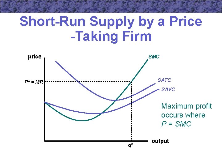
Short-Run Supply by a Price -Taking Firm price SMC SATC P* = MR SAVC Maximum profit occurs where P = SMC q* output

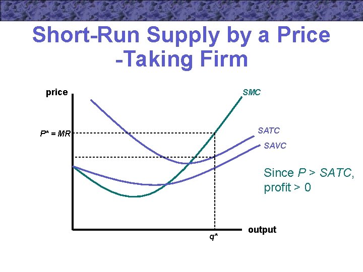
Short-Run Supply by a Price -Taking Firm price SMC SATC P* = MR SAVC Since P > SATC, profit > 0 q* output

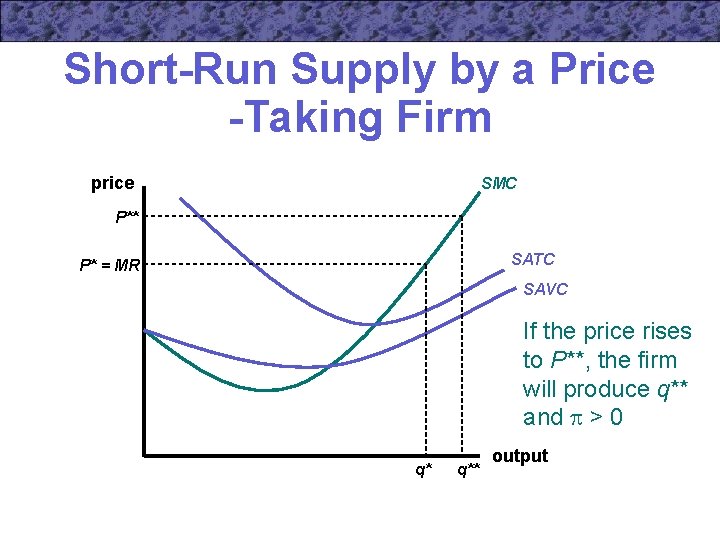
Short-Run Supply by a Price -Taking Firm price SMC P** SATC P* = MR SAVC If the price rises to P**, the firm will produce q** and > 0 q* q** output

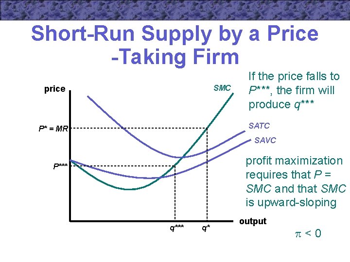
Short-Run Supply by a Price -Taking Firm SMC price If the price falls to P***, the firm will produce q*** SATC P* = MR SAVC profit maximization requires that P = SMC and that SMC is upward-sloping P*** q* output <0

Short-Run Supply by a Price -Taking Firm • The positively-sloped portion of the short-run marginal cost curve is the short-run supply curve for a price-taking firm – it shows how much the firm will produce at every possible market price – firms will only operate in the short run as long as total revenue covers variable cost • the firm will produce no output if P < SAVC

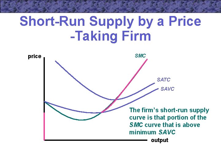
Short-Run Supply by a Price -Taking Firm • Thus, the price-taking firm’s short-run supply curve is the positively-sloped portion of the firm’s short-run marginal cost curve above the point of minimum average variable cost – for prices below this level, the firm’s profitmaximizing decision is to shut down and produce no output

Short-Run Supply by a Price -Taking Firm price SMC SATC SAVC The firm’s short-run supply curve is that portion of the SMC curve that is above minimum SAVC output

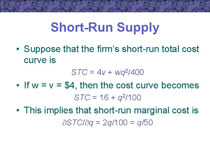
Short-Run Supply • Suppose that the firm’s short-run total cost curve is STC = 4 v + wq 2/400 • If w = v = $4, then the cost curve becomes STC = 16 + q 2/100 • This implies that short-run marginal cost is STC/ q = 2 q/100 = q/50

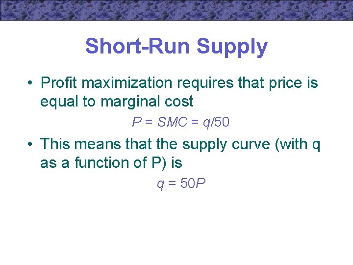
Short-Run Supply • Profit maximization requires that price is equal to marginal cost P = SMC = q/50 • This means that the supply curve (with q as a function of P) is q = 50 P

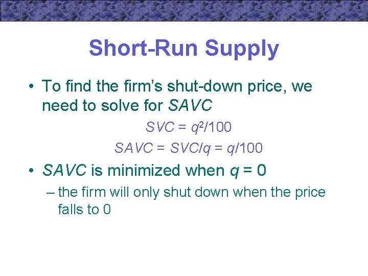
Short-Run Supply • To find the firm’s shut-down price, we need to solve for SAVC SVC = q 2/100 SAVC = SVC/q = q/100 • SAVC is minimized when q = 0 – the firm will only shut down when the price falls to 0

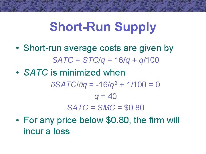
Short-Run Supply • Short-run average costs are given by SATC = STC/q = 16/q + q/100 • SATC is minimized when SATC/ q = -16/q 2 + 1/100 = 0 q = 40 SATC = SMC = $0. 80 • For any price below $0. 80, the firm will incur a loss

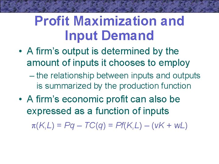
Profit Maximization and Input Demand • A firm’s output is determined by the amount of inputs it chooses to employ – the relationship between inputs and outputs is summarized by the production function • A firm’s economic profit can also be expressed as a function of inputs (K, L) = Pq – TC(q) = Pf(K, L) – (v. K + w. L)

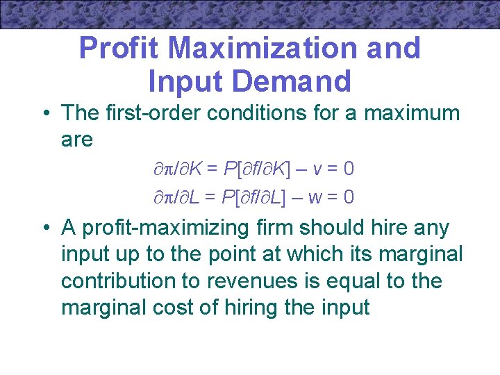
Profit Maximization and Input Demand • The first-order conditions for a maximum are / K = P[ f/ K] – v = 0 / L = P[ f/ L] – w = 0 • A profit-maximizing firm should hire any input up to the point at which its marginal contribution to revenues is equal to the marginal cost of hiring the input

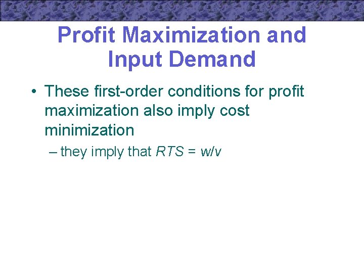
Profit Maximization and Input Demand • These first-order conditions for profit maximization also imply cost minimization – they imply that RTS = w/v

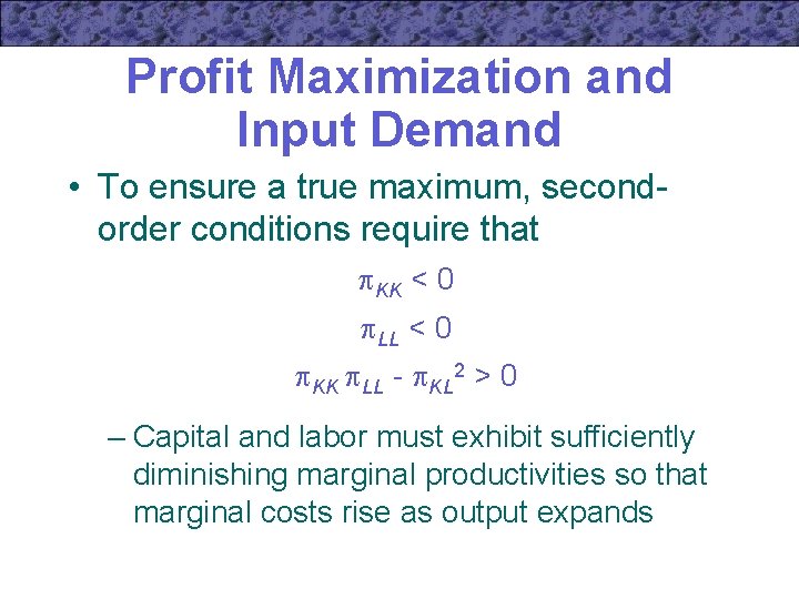
Profit Maximization and Input Demand • To ensure a true maximum, secondorder conditions require that KK < 0 LL < 0 KK LL - KL 2 > 0 – Capital and labor must exhibit sufficiently diminishing marginal productivities so that marginal costs rise as output expands

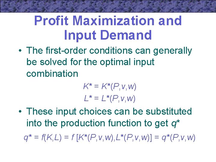
Profit Maximization and Input Demand • The first-order conditions can generally be solved for the optimal input combination K* = K*(P, v, w) L* = L*(P, v, w) • These input choices can be substituted into the production function to get q* q* = f(K, L) = f [K*(P, v, w), L*(P, v, w)] = q*(P, v, w)

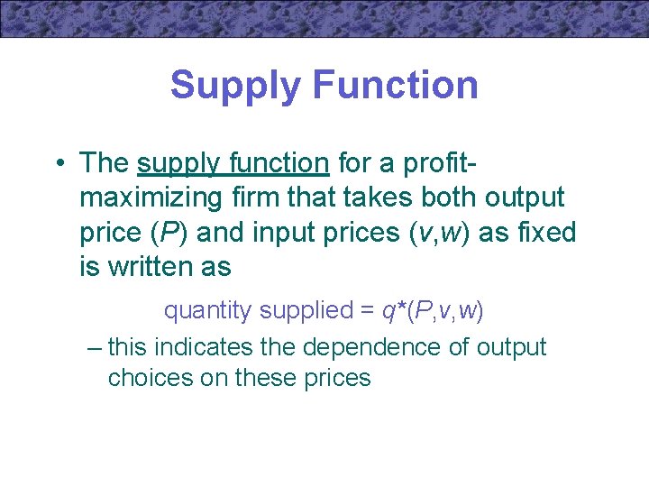
Supply Function • The supply function for a profitmaximizing firm that takes both output price (P) and input prices (v, w) as fixed is written as quantity supplied = q*(P, v, w) – this indicates the dependence of output choices on these prices

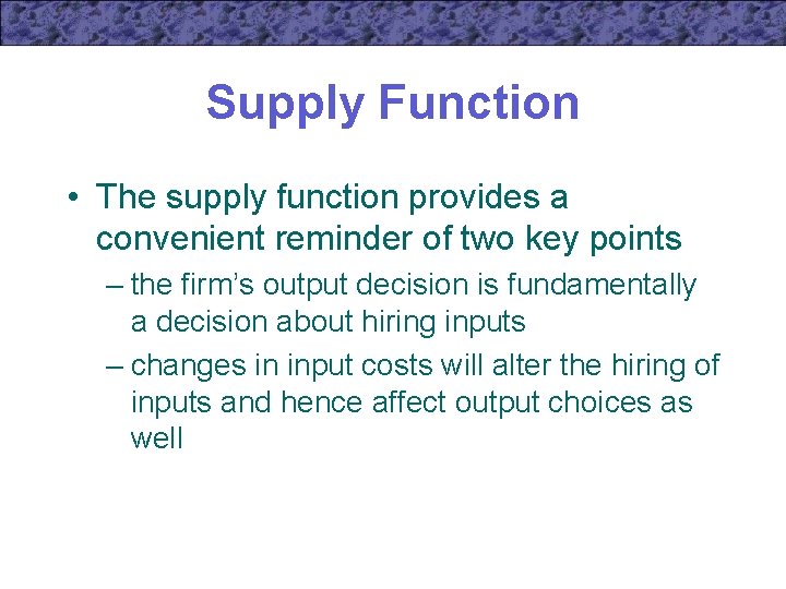
Supply Function • The supply function provides a convenient reminder of two key points – the firm’s output decision is fundamentally a decision about hiring inputs – changes in input costs will alter the hiring of inputs and hence affect output choices as well

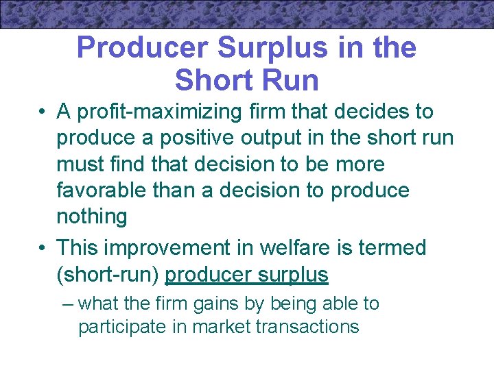
Producer Surplus in the Short Run • A profit-maximizing firm that decides to produce a positive output in the short run must find that decision to be more favorable than a decision to produce nothing • This improvement in welfare is termed (short-run) producer surplus – what the firm gains by being able to participate in market transactions

Producer Surplus in the Short Run • If the firm was prevented from making such transactions, output would be zero and profits would equal -SFC • Production of the profit-maximizing output would yield profits of * • The firm gains *+ SFC – this is producer surplus

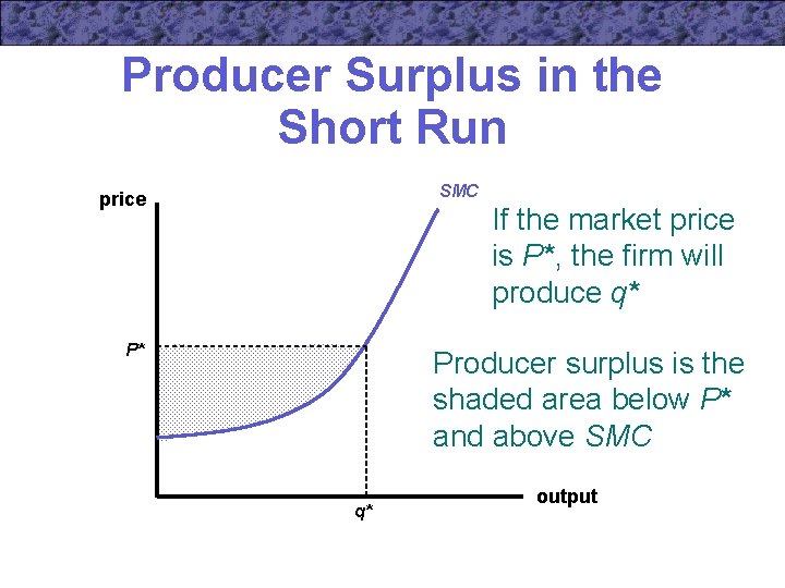
Producer Surplus in the Short Run SMC price If the market price is P*, the firm will produce q* P* Producer surplus is the shaded area below P* and above SMC q* output

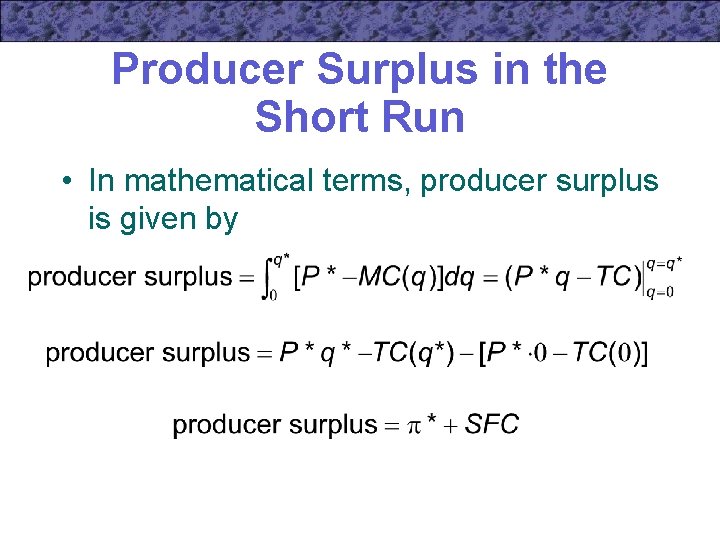
Producer Surplus in the Short Run • In mathematical terms, producer surplus is given by

Producer Surplus in the Short Run • Because SFC is constant, changes in producer surplus as a result of changes in market price are reflected as changes in short-run profits – these can be measured by the changes in the area below market price above the short-run supply curve

Producer Surplus in the Long Run • By definition, long-run producer surplus is zero – fixed costs do not exist in the long run – equilibrium profits under perfect competition with free entry are zero • In long-run analysis, attention is focused on the prices of the firm’s inputs and how they relate to what they would be in the absence of market transactions

Revenue Maximization • When firms are uncertain about the demand curve they face or when they have no reliable notion of the marginal costs of their output, the decision to maximize revenues may be a reasonable rule of thumb for ensuring their long-term survival

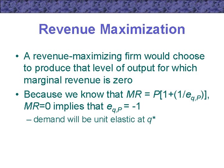
Revenue Maximization • A revenue-maximizing firm would choose to produce that level of output for which marginal revenue is zero • Because we know that MR = P[1+(1/eq, P)], MR=0 implies that eq, P = -1 – demand will be unit elastic at q*

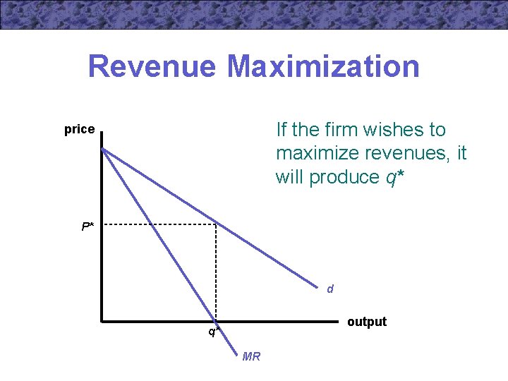
Revenue Maximization If the firm wishes to maximize revenues, it will produce q* price P* d output q* MR

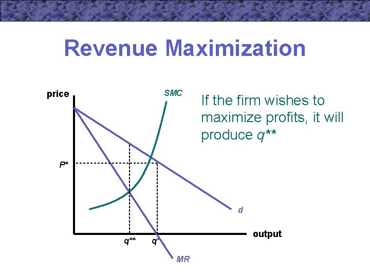
Revenue Maximization SMC price If the firm wishes to maximize profits, it will produce q** P* d q** output q* MR

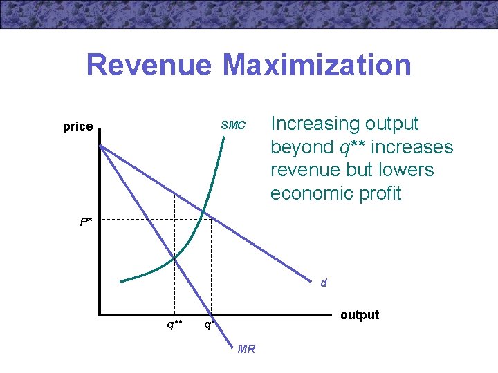
Revenue Maximization SMC price Increasing output beyond q** increases revenue but lowers economic profit P* d q** output q* MR

Constrained Revenue Maximization • A firm that chooses to maximize revenue is paying no attention to its costs – it is possible that maximizing revenues could result in negative profits for the firm • It may be more realistic to assume that these firms must meet some minimal level of profitability

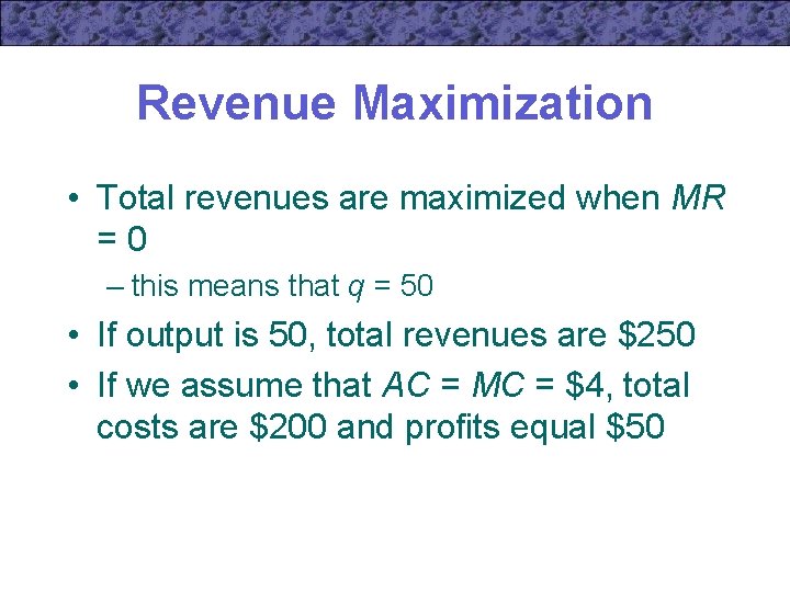
Revenue Maximization • Suppose that a firm faces the following demand curve q = 100 - 10 P • Total revenues (as a function of q) is TR = Pq = 10 q - q 2/10 • Marginal revenue is MR = d. TR/dq = 10 - q/5

Revenue Maximization • Total revenues are maximized when MR =0 – this means that q = 50 • If output is 50, total revenues are $250 • If we assume that AC = MC = $4, total costs are $200 and profits equal $50

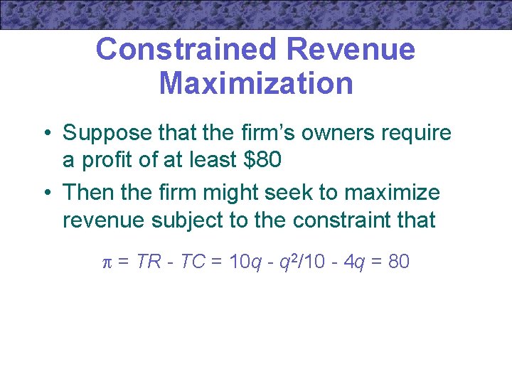
Constrained Revenue Maximization • Suppose that the firm’s owners require a profit of at least $80 • Then the firm might seek to maximize revenue subject to the constraint that = TR - TC = 10 q - q 2/10 - 4 q = 80

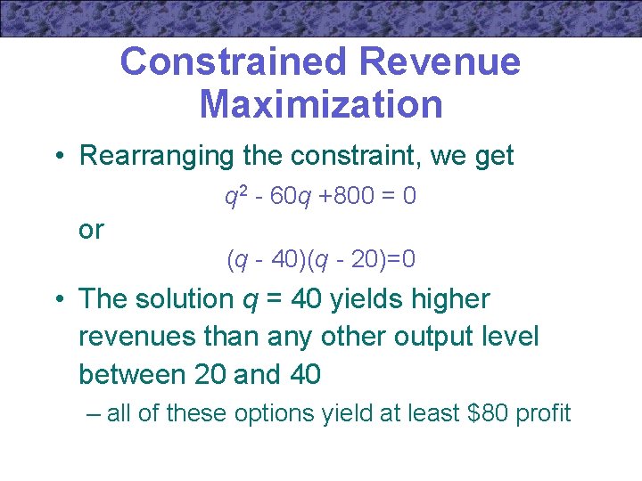
Constrained Revenue Maximization • Rearranging the constraint, we get q 2 - 60 q +800 = 0 or (q - 40)(q - 20)=0 • The solution q = 40 yields higher revenues than any other output level between 20 and 40 – all of these options yield at least $80 profit

The Principal-Agent Problem • In many cases, firm managers do not actually own the firm but instead act as agents for the owners • An agent is a person who makes economic decisions for another party

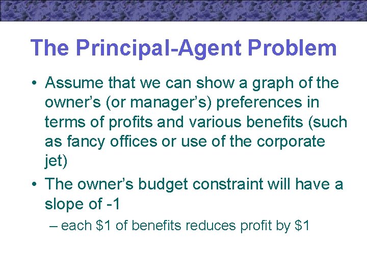
The Principal-Agent Problem • Assume that we can show a graph of the owner’s (or manager’s) preferences in terms of profits and various benefits (such as fancy offices or use of the corporate jet) • The owner’s budget constraint will have a slope of -1 – each $1 of benefits reduces profit by $1

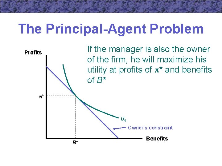
The Principal-Agent Problem If the manager is also the owner of the firm, he will maximize his utility at profits of * and benefits of B* Profits * U 1 Owner’s constraint B* Benefits

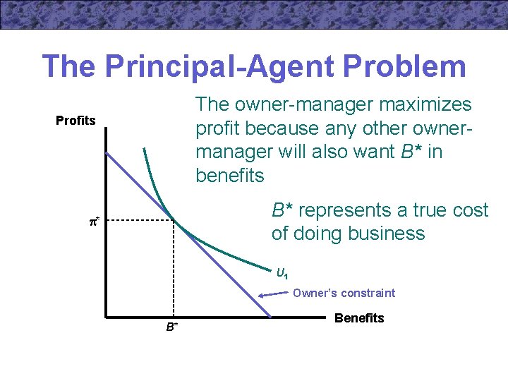
The Principal-Agent Problem The owner-manager maximizes profit because any other ownermanager will also want B* in benefits Profits B* represents a true cost of doing business * U 1 Owner’s constraint B* Benefits

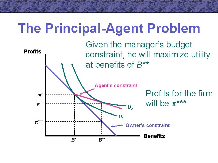
The Principal-Agent Problem • Suppose that the manager is not the sole owner of the firm – suppose there are two other owners who play no role in operating the firm • $1 in benefits only costs the manager $0. 33 in profits – the other $0. 67 is effectively paid by the other owners in terms of reduced profits

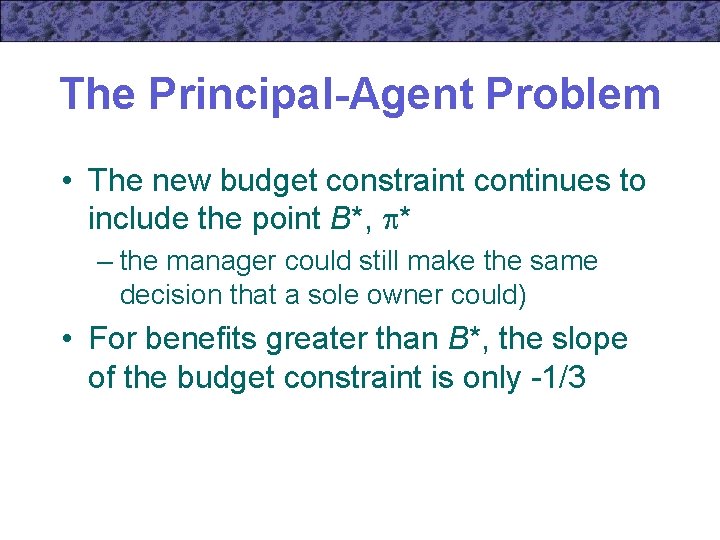
The Principal-Agent Problem • The new budget constraint continues to include the point B*, * – the manager could still make the same decision that a sole owner could) • For benefits greater than B*, the slope of the budget constraint is only -1/3

The Principal-Agent Problem Given the manager’s budget constraint, he will maximize utility at benefits of B** Profits Agent’s constraint * ** U 2 Profits for the firm will be *** U 1 *** Owner’s constraint B* B** Benefits

The Principal-Agent Problem • The firm’s owners are harmed by having to rely on an agency relationship with the firm’s manager • The smaller the fraction of the firm that is owned by the manager, the greater the distortions that will be induced by this relationship

The Principal-Agent Problem • The firm’s owners will not be happy about accepting lower profits on their investments – they may refuse to invest in the firm if they know the manager will behave in this manner • The manager could work out some contractual arrangement to induce the would-be owners to invest

The Principal-Agent Problem • One possible contract would be for the manager to agree to finance all of the benefits out of his share of the profits – results in lower utility for the manager – would be difficult to enforce • They may instead try to give managers an incentive to economize on benefits and to pursue higher profits

Important Points to Note: • In order to maximize profits, the firm should choose to produce that output level for which the marginal revenue is equal to the marginal cost • If a firm is a price taker, its output decisions do not affect the price of its output – marginal revenue is equal to price

Important Points to Note: • If the firm faces a downward-sloping demand for its output, it can only sell more at a lower price – marginal revenue will be less than price and may be negative • Marginal revenue and the price elasticity of demand are related by the following

Important Points to Note: • The supply curve for a price-taking, profitmaximizing firm is given by the positively sloped portion of its marginal cost curve above the point of minimum average variable cost – if price falls below minimum AVC, the firm’s profit-maximizing choice is to shut down and produce nothing

Important Points to Note: • The firm’s profit-maximization problem can also be approached as a problem in optimal input choice – this yields the same results as does an approach based on output choices • In the short run, firms obtain producer surplus in the form of short-run profits and coverage of fixed costs that would not be earned if the firm produced zero output

Important Points to Note: • In situations of imperfect knowledge, firms may opt to maximize revenues – this means that the firm expands output until marginal revenue is zero – sometimes these decisions may be constrained by minimum profit requirements • Because managers act as agents for a firm’s owners, they may not always make decisions that are consistent with profit maximization