Chapter 13 Binomial Trees 1 Binomial Trees Option

Chapter 13 Binomial Trees 1
 Binomial Approach -Advanced math -Cox, Ross and")
Binomial Trees Option pricing Model Black-Scholes (1973) Binomial Approach -Advanced math -Cox, Ross and Rubinstein (1979) -European option -Randleman and Bartter (1979) -Relatively simple -Both European and American option

One-period binomial option pricing model S=20
 is the ratio of the change in the price of a stock")
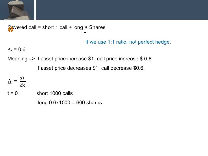
Delta (D) is the ratio of the change in the price of a stock option to the change in the price of the underlying stock The value of D varies from node to node Options, Futures, and Other Derivatives, 9 th Edition, Global Edition, Copyright © John C. Hull 2018 5

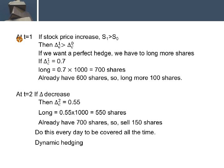
At : t = 1 If stock price increase $1, call price increase $0. 6 Short call => 1000 x -0. 6 = -600 Long stock => 600 x 1 Total profit = 600 0 If stock price decreases $1, call price decrease $0. 6. Short call => 1000 x 0. 6 = 600 Long stock => 600 x -1 = -600 Total profit 0

S=20 So, we will get 4. 5 for sure.

R=12% 4. 5 PV =?

Generalization A derivative lasts for time T and is dependent on a stock S 0 ƒ S 0 u ƒu S 0 d ƒd Options, Futures, and Other Derivatives, 9 th Edition, Global Edition, Copyright © John C. Hull 2018 11
 Value of a portfolio that is long D shares and short 1")
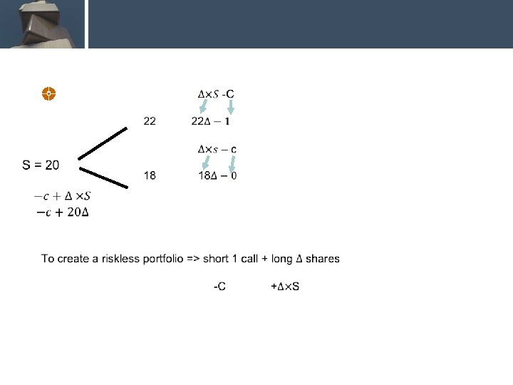
Generalization (continued) Value of a portfolio that is long D shares and short 1 derivative: S u. D – ƒ 0 u S 0 d. D – ƒd The portfolio is riskless when S 0 u. D – ƒu = S 0 d. D – ƒd or Options, Futures, and Other Derivatives, 9 th Edition, Global Edition, Copyright © John C. Hull 2018 12
 Value of the portfolio at time T is S 0 u. D")
Generalization (continued) Value of the portfolio at time T is S 0 u. D – ƒu Value of the portfolio today is (S 0 u. D – ƒu)e–r. T Another expression for the portfolio value today is S 0 D – f Hence ƒ = S 0 D – (S 0 u. D – ƒu )e–r. T Options, Futures, and Other Derivatives, 9 th Edition, Global Edition, Copyright © John C. Hull 2018 13
 Substituting for D we obtain ƒ = [ pƒu + (1 –")
Generalization (continued) Substituting for D we obtain ƒ = [ pƒu + (1 – p)ƒd ]e–r. T where Options, Futures, and Other Derivatives, 9 th Edition, Global Edition, Copyright © John C. Hull 2018 14

p as a Probability It is natural to interpret p and 1 -p as probabilities of up and down movements The value of a derivative is then its expected payoff in a risk-neutral world discounted at the risk-free rate S 0 ƒ p (1 – p) S 0 u ƒu S 0 d ƒd Options, Futures, and Other Derivatives, 9 th Edition, Global Edition, Copyright © John C. Hull 2018 15

Risk-Neutral Valuation When the probability of an up and down movements are p and 1 -p the expected stock price at time T is S 0 er. T This shows that the stock price earns the risk-free rate Binomial trees illustrate the general result that to value a derivative we can assume that the expected return on the underlying asset is the risk-free rate and discount at the risk-free rate This is known as using risk-neutral valuation Options, Futures, and Other Derivatives, 9 th Edition, Global Edition, Copyright © John C. Hull 2018 16

A Generalization S

20
)")
PV (E(port. T))

Risk-neutral probability P 1 -P O S T
 p= Only for non-dividend paying stock")
Risk – neutral probability (cont’) p= Only for non-dividend paying stock

How to use the above equation? R=12% 0

Two-Step binomial

3 P = 0. 652 22 P 1 -p= 034 3. 652 =0 1 -p =0 34 77 18 P . 6 =0 77 523 1 -p =0 34 77 0 12%

A Simple Binomial Model A stock price is currently $20 In 3 months it will be either $22 or $18 Stock Price = $22 Stock price = $20 Stock Price = $18 Options, Futures, and Other Derivatives, 9 th Edition, Global Edition, Copyright © John C. Hull 2018 26

A Call Option A 3 -month call option on the stock has a strike price of 21. Stock Price = $22 Option Price = $1 Stock price = $20 Option Price=? Stock Price = $18 Option Price = $0 Options, Futures, and Other Derivatives, 9 th Edition, Global Edition, Copyright © John C. Hull 2018 27

Valuing the Option The portfolio that is long 0. 25 shares short 1 option is worth 4. 367 The value of the shares is 5. 000 (= 0. 25 × 20 ) The value of the option is therefore 0. 633 ( 5. 000 – 0. 633 = 4. 367 ) Options, Futures, and Other Derivatives, 9 th Edition, Global Edition, Copyright © John C. Hull 2018 28
 S 0 u =")
Original Example Revisited p S 0=20 ƒ (1 – p) S 0 u = 22 ƒu = 1 S 0 d = 18 ƒd = 0 p is the probability that gives a return on the stock equal to the risk-free rate: 20 e 0. 12 × 0. 25 = 22 p + 18(1 – p ) so that p = 0. 6523 Alternatively: Options, Futures, and Other Derivatives, 9 th Edition, Global Edition, Copyright © John C. Hull 2018 29

Valuing the Option Using Risk-Neutral Valuation 23 0. 65 S 0=20 ƒ 0. 34 77 S 0 u = 22 ƒu = 1 S 0 d = 18 ƒd = 0 The value of the option is e– 0. 12× 0. 25 (0. 6523× 1 + 0. 3477× 0) = 0. 633 Options, Futures, and Other Derivatives, 9 th Edition, Global Edition, Copyright © John C. Hull 2018 30

Irrelevance of Stock’s Expected Return When we are valuing an option in terms of the price of the underlying asset, the probability of up and down movements in the real world are irrelevant This is an example of a more general result stating that the expected return on the underlying asset in the real world is irrelevant Options, Futures, and Other Derivatives, 9 th Edition, Global Edition, Copyright © John C. Hull 2018 31

A Two-Step Example Figure 13. 3, page 303 24. 2 22 19. 8 20 18 K=21, r = 12% Each time step is 3 months 16. 2 Options, Futures, and Other Derivatives, 9 th Edition, Global Edition, Copyright © John C. Hull 2018 32

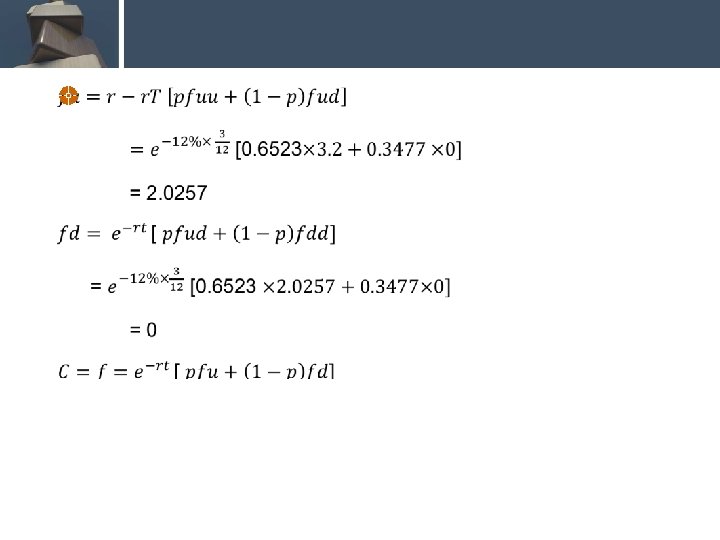
Valuing a Call Option Figure 13. 4, page 303 22 20 1. 2823 2. 0257 A 18 0. 0 24. 2 3. 2 B 19. 8 0. 0 16. 2 0. 0 Value at node B = e– 0. 12× 0. 25(0. 6523× 3. 2 + 0. 3477× 0) = 2. 0257 Value at node A = e– 0. 12× 0. 25(0. 6523× 2. 0257 + 0. 3477× 0) = 1. 2823 Options, Futures, and Other Derivatives, 9 th Edition, Global Edition, Copyright © John C. Hull 2018 33

A Put Option Example 50 4. 1923 60 1. 4147 40 9. 4636 72 0 48 4 32 20 K = 52, time step =1 yr r = 5%, u =1. 32, d = 0. 8, p = 0. 6282 Options, Futures, and Other Derivatives, 9 th Edition, Global Edition, Copyright © John C. Hull 2018 34
 72")
What Happens When the Put Option is American (Figure 13. 8, page 307) 72 0 60 50 5. 0894 The American feature increases the value at node C from 9. 4636 to 12. 0000. 48 4 1. 4147 40 12. 0 C 32 20 This increases the value of the option from 4. 1923 to 5. 0894. Options, Futures, and Other Derivatives, 9 th Edition, Global Edition, Copyright © John C. Hull 2018 35

Choosing u and d One way of matching the volatility is to set where s is the volatility and Dt is the length of the time step. This is the approach used by Cox, Ross, and Rubinstein Options, Futures, and Other Derivatives, 9 th Edition, Global Edition, Copyright © John C. Hull 2018 36

Girsanov’s Theorem Volatility is the same in the real world and the risk-neutral world We can therefore measure volatility in the real world and use it to build a tree for the an asset in the risk-neutral world Options, Futures, and Other Derivatives, 9 th Edition, Global Edition, Copyright © John C. Hull 2018 37

Assets Other than Non-Dividend Paying Stocks For options on stock indices, currencies and futures the basic procedure for constructing the tree is the same except for the calculation of p Options, Futures, and Other Derivatives, 9 th Edition, Global Edition, Copyright © John C. Hull 2018 38

The Probability of an Up Move Options, Futures, and Other Derivatives, 9 th Edition, Global Edition, Copyright © John C. Hull 2018 39
- Slides: 39