Chapter 12 SUPERVISED LEARNING Rule Algorithms and their
![CLIP 4 Algorithm Phase 1: Use the first negative example [1, 3, 2, 1] CLIP 4 Algorithm Phase 1: Use the first negative example [1, 3, 2, 1]](https://slidetodoc.com/presentation_image_h2/8875634fae7fb698930601eb1fcfb110/image-26.jpg)
- Slides: 75

Chapter 12 SUPERVISED LEARNING Rule Algorithms and their Hybrids Part 2 Cios / Pedrycz / Swiniarski / Kurgan

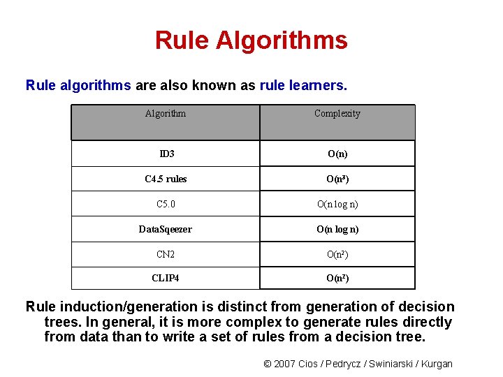
Rule Algorithms Rule algorithms are also known as rule learners. Algorithm Complexity ID 3 O(n) C 4. 5 rules O(n 3) C 5. 0 O(n log n) Data. Sqeezer O(n log n) CN 2 O(n 2) CLIP 4 O(n 2) Rule induction/generation is distinct from generation of decision trees. In general, it is more complex to generate rules directly from data than to write a set of rules from a decision tree. © 2007 Cios / Pedrycz / Swiniarski / Kurgan

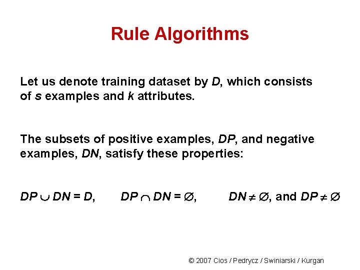
Rule Algorithms Let us denote training dataset by D, which consists of s examples and k attributes. The subsets of positive examples, DP, and negative examples, DN, satisfy these properties: DP DN = D, DP DN = , DN , and DP © 2007 Cios / Pedrycz / Swiniarski / Kurgan

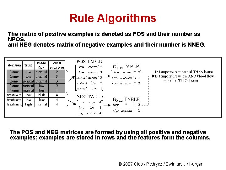
Rule Algorithms The matrix of positive examples is denoted as POS and their number as NPOS, and NEG denotes matrix of negative examples and their number is NNEG. The POS and NEG matrices are formed by using all positive and negative examples; examples are stored in rows and the features form the columns. © 2007 Cios / Pedrycz / Swiniarski / Kurgan

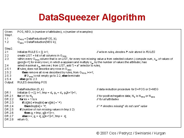
Data. Squeezer Algorithm Given: Step 1. 1. 1 1. 2 Step 2. 2. 1 2. 2 2. 3 POS, NEG, k (number of attributes), s (number of examples) GPOS = Data. Reduction(POS, k); GNEG = Data. Reduction(NEG k); 2. 4 2. 5. 1 2. 5. 2 2. 5. 3 2. 5. 4 Output: Initialize RULES = []; i=1; // where rulesi denotes ith rule stored in RULES create LIST = list of all columns in GPOS within every GPOS column that is on LIST, for every non missing value a from selected column j compute sum, saj, of values of gposi[k+1] for every row i, in which a appears and multiply saj, by the number of values the attribute j has select maximal saj, remove j from LIST, add “j = a” selector to rulesi if rulesi does not describe any rows in GNEG then remove all rows described by rulesi from GPOS, i=i+1; if GPOS is not empty go to 2. 2, else terminate else go to 2. 3 RULES describing POS DR. 1 DR. 2. 2 DR. 2. 3 DR. 2. 4 DR. 2. 5 DR. 2. 6 DR. 2. 7 DR. 2. 8 Data. Reduction (D, k) Initialize G = []; i=1; tmp = d 1; g 1[k+1]=1; for j=1 to ND for kk = 1 to k if (dj[kk] tmp[kk] or dj[kk] = ‘ ’) then tmp[kk] = ‘ ’; if (number of non missing values in tmp 2) then gi = tmp; gi[k+1]++; else i++; gi = dj; gi[k+1]=1; tmp = dj; return G; // data reduction procedure for D=POS or D=NEG // for positive/negative data; ND is NPOS or NNEG // for all attributes // ‘ ’ denotes missing” do not care” value © 2007 Cios / Pedrycz / Swiniarski / Kurgan

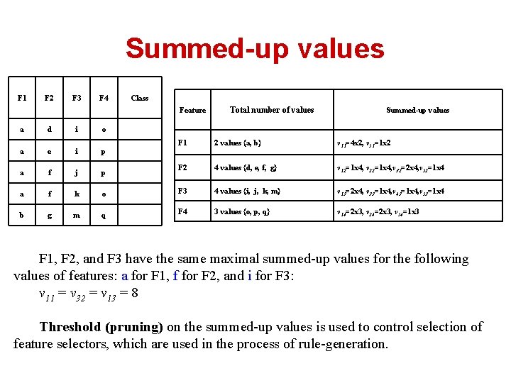
Summed-up values F 1 F 2 F 3 F 4 Class Feature a d i o a e i p a f j p a f k b g m Total number of values Summed-up values F 1 2 values {a, b} v 11=4 x 2, v 51=1 x 2 F 2 4 values {d, e, f, g} v 12=1 x 4, v 22=1 x 4, v 32=2 x 4, v 52=1 x 4 o F 3 4 values {i, j, k, m} v 13=2 x 4, v 33=1 x 4, v 43=1 x 4, v 53=1 x 4 q F 4 3 values {o, p, q} v 14=2 x 3, v 24=2 x 3, v 54=1 x 3 F 1, F 2, and F 3 have the same maximal summed-up values for the following values of features: a for F 1, f for F 2, and i for F 3: v 11 = v 32 = v 13 = 8 Threshold (pruning) on the summed-up values is used to control selection of feature selectors, which are used in the process of rule-generation.

© 2007 Cios / Pedrycz / Swiniarski / Kurgan

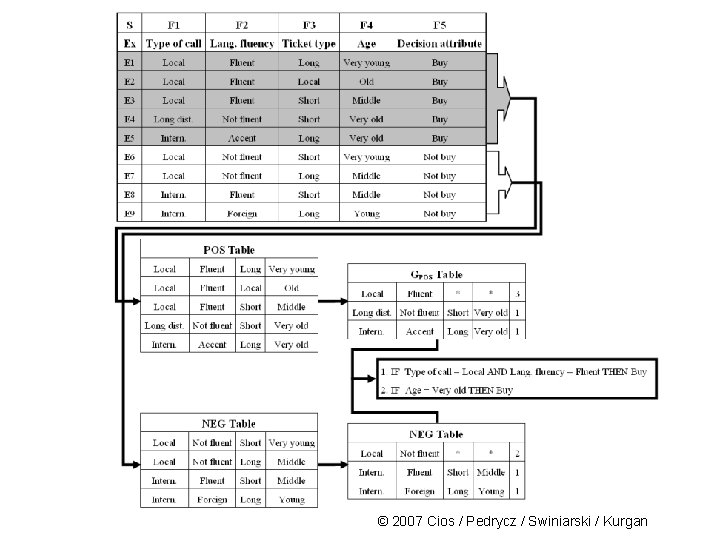
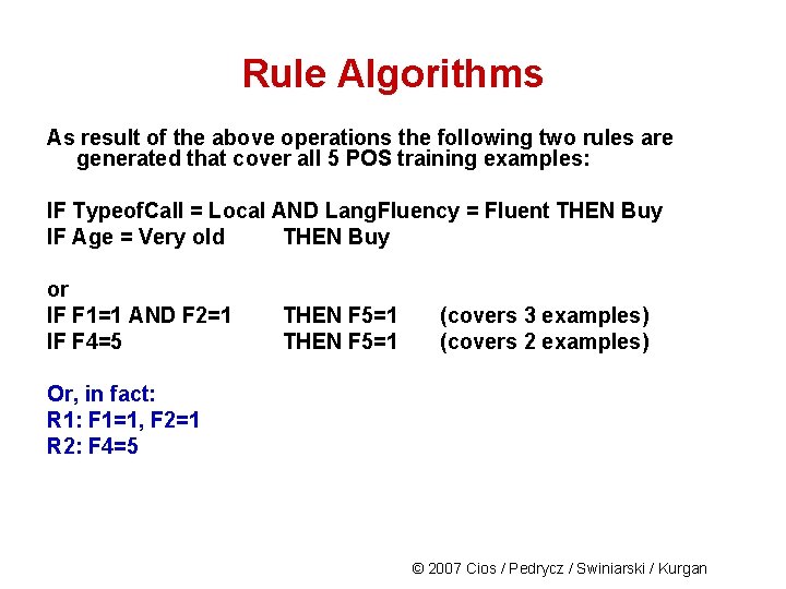
Rule Algorithms As result of the above operations the following two rules are generated that cover all 5 POS training examples: IF Typeof. Call = Local AND Lang. Fluency = Fluent THEN Buy IF Age = Very old THEN Buy or IF F 1=1 AND F 2=1 IF F 4=5 THEN F 5=1 (covers 3 examples) (covers 2 examples) Or, in fact: R 1: F 1=1, F 2=1 R 2: F 4=5 © 2007 Cios / Pedrycz / Swiniarski / Kurgan

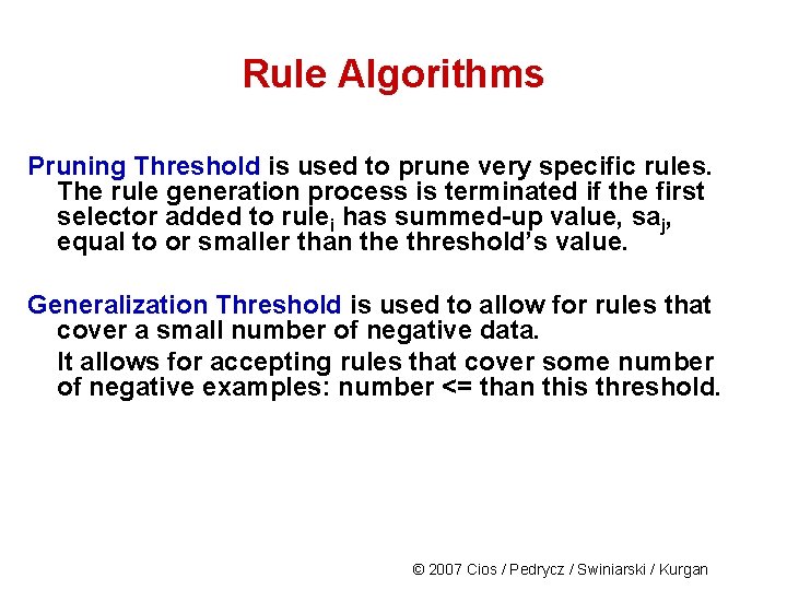
Rule Algorithms Pruning Threshold is used to prune very specific rules. The rule generation process is terminated if the first selector added to rulei has summed-up value, saj, equal to or smaller than the threshold’s value. Generalization Threshold is used to allow for rules that cover a small number of negative data. It allows for accepting rules that cover some number of negative examples: number <= than this threshold. © 2007 Cios / Pedrycz / Swiniarski / Kurgan

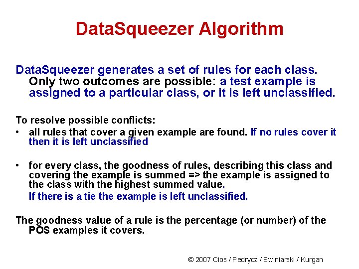
Data. Squeezer Algorithm Data. Squeezer generates a set of rules for each class. Only two outcomes are possible: a test example is assigned to a particular class, or it is left unclassified. To resolve possible conflicts: • all rules that cover a given example are found. If no rules cover it then it is left unclassified • for every class, the goodness of rules, describing this class and covering the example is summed => the example is assigned to the class with the highest summed value. If there is a tie the example is left unclassified. The goodness value of a rule is the percentage (or number) of the POS examples it covers. © 2007 Cios / Pedrycz / Swiniarski / Kurgan

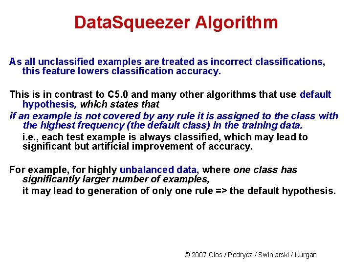
Data. Squeezer Algorithm As all unclassified examples are treated as incorrect classifications, this feature lowers classification accuracy. This is in contrast to C 5. 0 and many other algorithms that use default hypothesis, which states that if an example is not covered by any rule it is assigned to the class with the highest frequency (the default class) in the training data. i. e. , each test example is always classified, which may lead to significant but artificial improvement of accuracy. For example, for highly unbalanced data, where one class has significantly larger number of examples, it may lead to generation of only one rule => the default hypothesis. © 2007 Cios / Pedrycz / Swiniarski / Kurgan

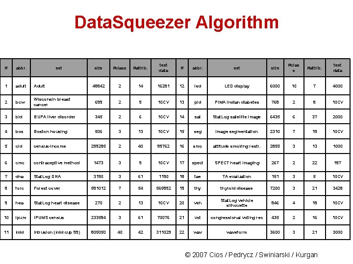
Data. Squeezer Algorithm size #class #attrib. test data # abbr. set size #clas s #attrib. test data 48842 2 14 16281 12 led LED display 6000 10 7 4000 Wisconsin breast cancer 699 2 9 10 CV 13 pid PIMA indian diabetes 768 2 8 10 CV bld BUPA liver disorder 345 2 6 10 CV 14 sat Stat. Log satellite image 6435 6 37 2000 4 bos Boston housing 506 3 13 10 CV 15 seg image segmentation 2310 7 19 10 CV 5 cid census-income 299285 2 40 99762 16 smo attitude smoking restr. 2855 3 13 1000 6 cmc contraceptive method 1473 3 9 10 CV 17 spect SPECT heart imaging 267 2 22 187 7 dna Stat. Log DNA 3190 3 61 1190 18 tae TA evaluation 151 3 5 10 CV 8 forc Forest cover 581012 7 54 565892 19 thyroid disease 7200 3 21 3428 9 hea Stat. Log heart disease 270 2 13 10 CV 20 veh Stat. Log vehicle silhouette 846 4 18 10 CV 10 ipum IPUMS census 233584 3 61 70076 21 vot congressional voting rec 435 2 16 10 CV 11 kdd Intrusion (kdd cup 99) 805050 40 42 311029 22 waveform 3600 3 21 3000 # abbr. set 1 adult Adult 2 bcw 3 © 2007 Cios / Pedrycz / Swiniarski / Kurgan

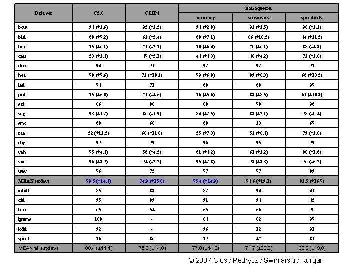
Data set C 5. 0 CLIP 4 bcw 94 (± 2. 6) bld Data. Squeezer accuracy sensitivity specificity 95 (± 2. 5) 94 (± 2. 8) 92 (± 3. 5) 98 (± 3. 3) 68 (± 7. 2) 63 (± 5. 4) 68 (± 7. 1) 86 (± 18. 5) 44 (± 21. 5) bos 75 (± 6. 1) 71 (± 2. 7) 70 (± 6. 4) 70 (± 6. 1) 88 (± 4. 3) cmc 53 (± 3. 4) 47 (± 5. 1) 44 (± 4. 3) 40 (± 4. 2) 73 (± 2. 0) dna 94 91 92 92 97 hea 78 (± 7. 6) 72 (± 10. 2) 79 (± 6. 0) 89 (± 8. 3) 66 (± 13. 5) led 74 71 68 68 97 pid 75 (± 5. 0) 71 (± 4. 5) 76 (± 5. 6) 83 (± 8. 5) 61 (± 10. 3) sat 86 80 80 78 96 seg 93 (± 1. 2) 86 (± 1. 9) 84 (± 2. 5) 83 (± 2. 1) 98 (± 0. 4) smo 68 68 68 33 67 tae 52 (± 12. 5) 60 (± 11. 8) 55 (± 7. 3) 53 (± 8. 4) 79 (± 3. 8) thy 99 99 96 95 99 veh 75 (± 4. 4) 56 (± 4. 5) 61 (± 4. 2) 61 (± 3. 2) 88 (± 1. 6) vot 96 (± 3. 9) 94 (± 2. 2) 95 (± 2. 8) 93 (± 3. 3) 96 (± 5. 2) wav 76 75 77 77 89 78. 5 (± 14. 4) 74. 9 (± 15. 0) 75. 4 (± 14. 9) 74. 6 (± 19. 1) 83. 5 (± 16. 7) adult 85 83 82 94 41 cid 95 89 91 94 45 forc 65 54 55 56 90 ipums 100 - 84 82 97 kdd 92 - 96 12 91 spect 76 86 79 47 81 80. 4 (± 14. 1) 75. 6 (± 14. 8) 77. 0 (± 14. 6) 71. 7 (± 23. 0) 80. 9 (± 19. 0) MEAN (stdev) MEAN all (stdev) © 2007 Cios / Pedrycz / Swiniarski / Kurgan

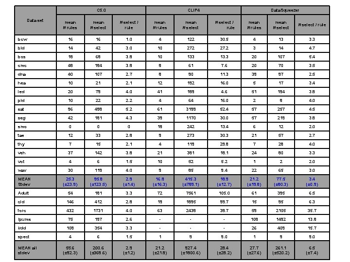
C 5. 0 Data set CLIP 4 Data. Squeezer mean # rules mean # select / rule mean # rules mean # select / rule bcw 16 16 1. 0 4 122 30. 5 4 13 3. 3 bld 14 42 3. 0 10 272 27. 2 3 14 4. 7 bos 18 68 3. 8 10 133 13. 3 20 107 5. 4 cmc 48 184 3. 8 8 61 7. 6 20 70 3. 5 dna 40 107 2. 7 8 90 11. 3 39 97 2. 5 hea 10 21 2. 1 12 192 16. 0 5 17 3. 4 led 20 79 4. 0 41 189 4. 6 51 194 3. 8 pid 10 22 2. 2 4 64 16. 0 2 8 4. 0 sat 96 498 5. 2 61 3199 52. 4 57 257 4. 5 seg 42 181 4. 3 39 1170 30. 0 57 219 3. 8 smo 0 0 0 18 242 13. 4 6 12 2. 0 tae 12 33 2. 8 9 273 30. 3 21 57 2. 7 thy 7 15 2. 1 4 119 29. 8 7 28 4. 0 veh 37 142 3. 8 21 381 18. 1 24 80 3. 3 vot 4 6 1. 5 10 52 5. 2 1 2 2. 0 wav 30 119 4. 0 9 85 9. 4 22 65 3. 0 MEAN Stdev 25. 3 (± 23. 9) 95. 8 (± 123. 5) 2. 9 (± 1. 4) 16. 8 (± 16. 3) 415. 3 (± 789. 1) 18. 9 (± 12. 7) 21. 2 (± 19. 8) 77. 5 (± 80. 3) 3. 4 (± 0. 9) Adult 54 181 3. 3 72 7561 105. 0 61 395 6. 5 cid 146 412 2. 8 19 1895 99. 7 15 95 6. 3 forc 432 1731 4. 0 63 2438 38. 7 59 2105 35. 7 Ipums 75 197 2. 6 - - - 108 1492 13. 8 kdd 108 354 3. 3 - - - 26 409 15. 7 4 6 1. 5 1 9 9. 0 55. 6 (± 92. 3) 200. 6 (± 368. 6) 2. 9 (± 1. 2) 21. 2 (± 21. 8) 28. 4 27. 7 261. 1 6. 5 spect MEAN all stdev 927. 4 (± 1800. 6) © 2007 (± 28. 2) (± 27. 6) (± 520. 2) / Kurgan (± 7. 4) Cios / Pedrycz / Swiniarski

Hybrid Algorithms • A hybrid algorithm combines methods from two or more types of algorithms • The goal of a hybrid algorithm design is to combine the most useful mechanisms of two or more algorithms to achieve better robustness, speed, accuracy, etc. © 2007 Cios / Pedrycz / Swiniarski / Kurgan

Hybrid Algorithms Hybrid algorithms that combine decision trees and rule algorithms: - CN 2 algorithm (Clark and Niblett, 1989) - CLIP algorithms CLILP 2 (Cios and Liu, 1995) CLIP 3 (Cios, Wedding and Liu, 1997) CLIP 4 (Cios and Kurgan, 2004) © 2007 Cios / Pedrycz / Swiniarski / Kurgan

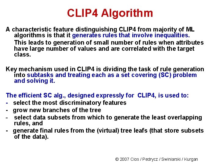
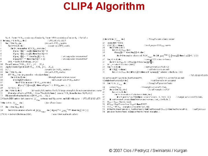
CLIP 4 Algorithm A characteristic feature distinguishing CLIP 4 from majority of ML algorithms is that it generates rules that involve inequalities. This leads to generation of small number of rules when attributes have large number of values and are correlated with the target class. Key mechanism used in CLIP 4 is dividing the task of rule generation into subtasks and treating each as a set covering (SC) problem and solving it. The efficient SC alg. , designed expressly for CLIP 4, is used to: - select the most discriminatory features - grow new branches of the tree - select data subsets from which to generate the least overlapping rules, and - generate final rules from the (virtual) tree leafs (that store subsets of the data). © 2007 Cios / Pedrycz / Swiniarski / Kurgan

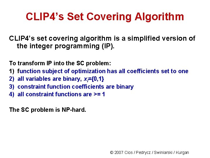
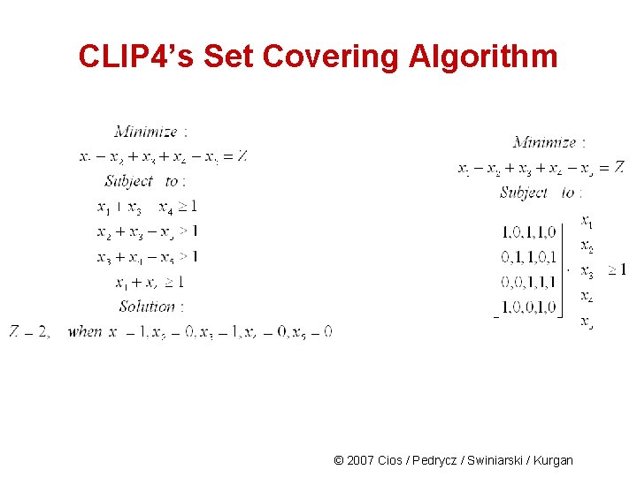
CLIP 4’s Set Covering Algorithm CLIP 4’s set covering algorithm is a simplified version of the integer programming (IP). To transform IP into the SC problem: 1) function subject of optimization has all coefficients set to one 2) all variables are binary, xi={0, 1} 3) constraint function coefficients are binary 4) all constraint functions are >= 1 The SC problem is NP-hard. © 2007 Cios / Pedrycz / Swiniarski / Kurgan

CLIP 4’s Set Covering Algorithm © 2007 Cios / Pedrycz / Swiniarski / Kurgan

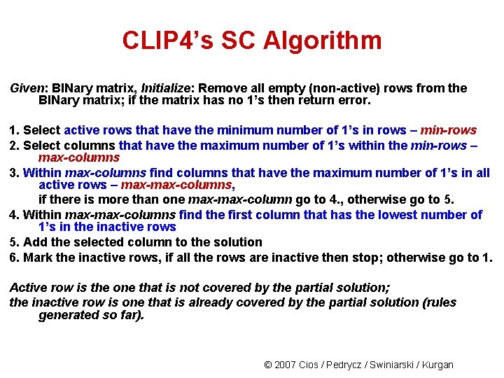
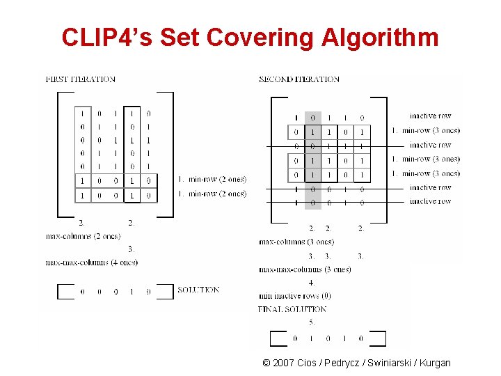
CLIP 4’s SC Algorithm Given: BINary matrix, Initialize: Remove all empty (non-active) rows from the BINary matrix; if the matrix has no 1’s then return error. 1. Select active rows that have the minimum number of 1’s in rows – min-rows 2. Select columns that have the maximum number of 1’s within the min-rows – max-columns 3. Within max-columns find columns that have the maximum number of 1’s in all active rows – max-columns, if there is more than one max-column go to 4. , otherwise go to 5. 4. Within max-columns find the first column that has the lowest number of 1’s in the inactive rows 5. Add the selected column to the solution 6. Mark the inactive rows, if all the rows are inactive then stop; otherwise go to 1. Active row is the one that is not covered by the partial solution; the inactive row is one that is already covered by the partial solution (rules generated so far). © 2007 Cios / Pedrycz / Swiniarski / Kurgan

CLIP 4’s Set Covering Algorithm © 2007 Cios / Pedrycz / Swiniarski / Kurgan

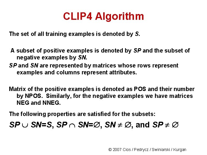
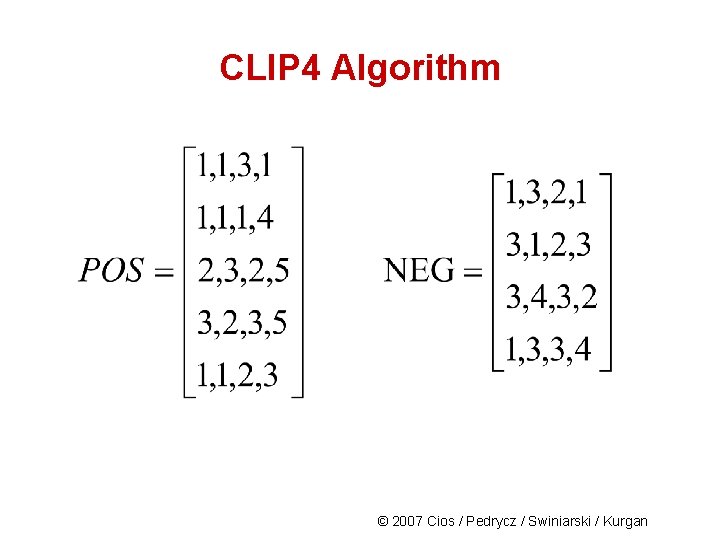
CLIP 4 Algorithm The set of all training examples is denoted by S. A subset of positive examples is denoted by SP and the subset of negative examples by SN. SP and SN are represented by matrices whose rows represent examples and columns represent attributes. Matrix of the positive examples is denoted as POS and their number by NPOS. Similarly, for the negative examples we have matrices NEG and NNEG. The following properties are satisfied for the subsets: SP SN=S, SP SN= , SN , and SP © 2007 Cios / Pedrycz / Swiniarski / Kurgan

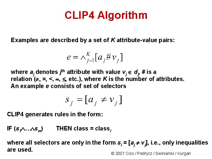
CLIP 4 Algorithm Examples are described by a set of K attribute-value pairs: where aj denotes jth attribute with value vj dj, # is a relation ( , =, <, , , etc. ), where K is the number of attributes. An example e consists of set of selectors CLIP 4 generates rules in the form: IF (s 1 … sm) THEN class = classi where all selectors are only in the form si = [aj vj], i. e. , only inequalities are used. © 2007 Cios / Pedrycz / Swiniarski / Kurgan

CLIP 4 Algorithm 1 © 2007 Cios / Pedrycz / Swiniarski / Kurgan

CLIP 4 Algorithm © 2007 Cios / Pedrycz / Swiniarski / Kurgan
![CLIP 4 Algorithm Phase 1 Use the first negative example 1 3 2 1 CLIP 4 Algorithm Phase 1: Use the first negative example [1, 3, 2, 1]](https://slidetodoc.com/presentation_image_h2/8875634fae7fb698930601eb1fcfb110/image-26.jpg)
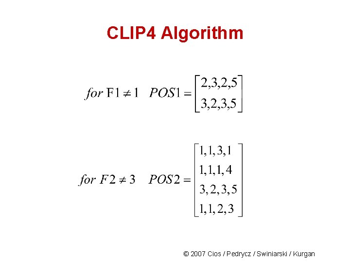
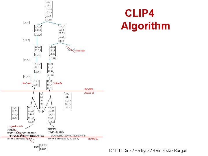
CLIP 4 Algorithm Phase 1: Use the first negative example [1, 3, 2, 1] and matrix POS to create the BINARY matrix © 2007 Cios / Pedrycz / Swiniarski / Kurgan

CLIP 4 Algorithm © 2007 Cios / Pedrycz / Swiniarski / Kurgan

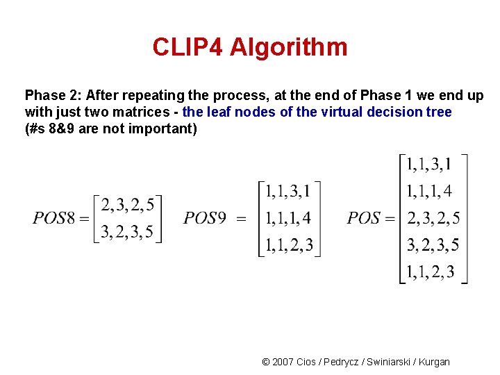
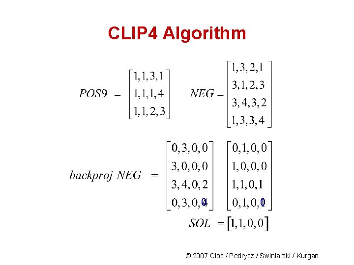
CLIP 4 Algorithm Phase 2: After repeating the process, at the end of Phase 1 we end up with just two matrices - the leaf nodes of the virtual decision tree (#s 8&9 are not important) © 2007 Cios / Pedrycz / Swiniarski / Kurgan

CLIP 4 Algorithm © 2007 Cios / Pedrycz / Swiniarski / Kurgan

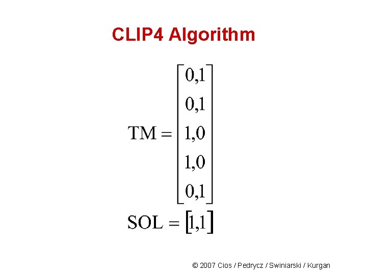
CLIP 4 Algorithm 0 0 © 2007 Cios / Pedrycz / Swiniarski / Kurgan

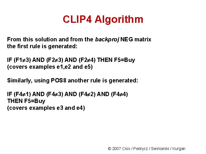
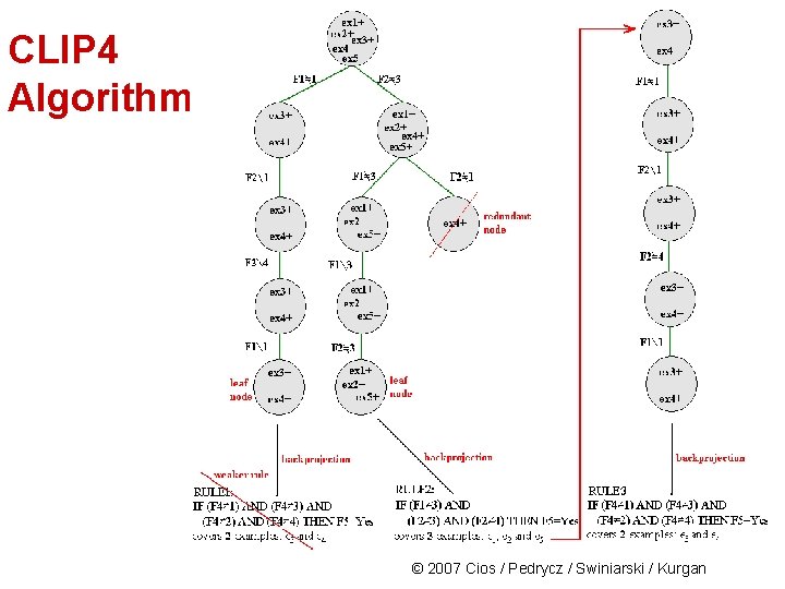
CLIP 4 Algorithm From this solution and from the backproj NEG matrix the first rule is generated: IF (F 1 3) AND (F 2 4) THEN F 5=Buy (covers examples e 1, e 2 and e 5) Similarly, using POS 8 another rule is generated: IF (F 4 1) AND (F 4 3) AND (F 4 2) AND (F 4 4) THEN F 5=Buy (covers examples e 3 and e 4) © 2007 Cios / Pedrycz / Swiniarski / Kurgan

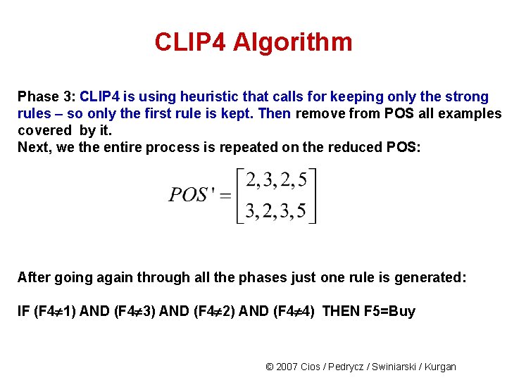
CLIP 4 Algorithm Phase 3: CLIP 4 is using heuristic that calls for keeping only the strong rules – so only the first rule is kept. Then remove from POS all examples covered by it. Next, we the entire process is repeated on the reduced POS: After going again through all the phases just one rule is generated: IF (F 4 1) AND (F 4 3) AND (F 4 2) AND (F 4 4) THEN F 5=Buy © 2007 Cios / Pedrycz / Swiniarski / Kurgan

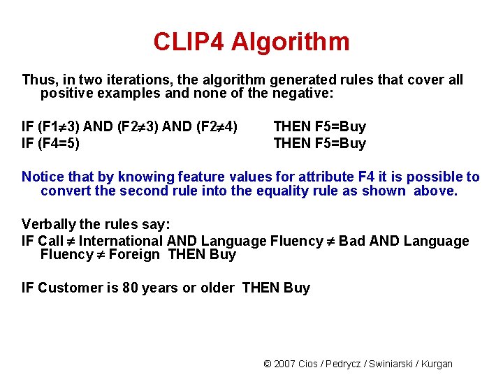
CLIP 4 Algorithm Thus, in two iterations, the algorithm generated rules that cover all positive examples and none of the negative: IF (F 1 3) AND (F 2 4) IF (F 4=5) THEN F 5=Buy Notice that by knowing feature values for attribute F 4 it is possible to convert the second rule into the equality rule as shown above. Verbally the rules say: IF Call International AND Language Fluency Bad AND Language Fluency Foreign THEN Buy IF Customer is 80 years or older THEN Buy © 2007 Cios / Pedrycz / Swiniarski / Kurgan

CLIP 4 Algorithm © 2007 Cios / Pedrycz / Swiniarski / Kurgan

CLIP 4 Algorithm © 2007 Cios / Pedrycz / Swiniarski / Kurgan

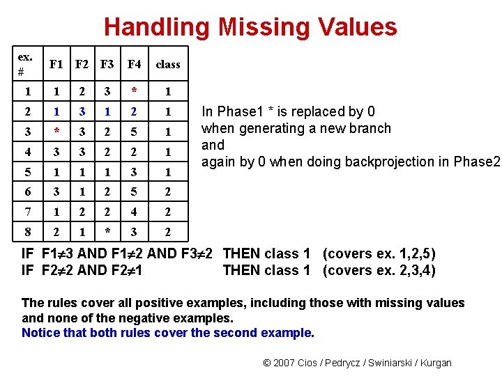
Handling Missing Values ex. # F 1 F 2 F 3 F 4 class 1 1 2 3 * 1 2 1 3 * 3 2 5 1 4 3 3 2 2 1 5 1 1 1 3 1 6 3 1 2 5 2 7 1 2 2 4 2 8 2 1 * 3 2 In Phase 1 * is replaced by 0 when generating a new branch and again by 0 when doing backprojection in Phase 2 IF F 1 3 AND F 1 2 AND F 3 2 THEN class 1 (covers ex. 1, 2, 5) IF F 2 2 AND F 2 1 THEN class 1 (covers ex. 2, 3, 4) The rules cover all positive examples, including those with missing values and none of the negative examples. Notice that both rules cover the second example. © 2007 Cios / Pedrycz / Swiniarski / Kurgan

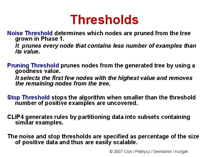
Thresholds Noise Threshold determines which nodes are pruned from the tree grown in Phase 1. It prunes every node that contains less number of examples than its value. Pruning Threshold prunes nodes from the generated tree by using a goodness value. It selects the first few nodes with the highest value and removes the remaining nodes from the tree. Stop Threshold stops the algorithm when smaller than the threshold number of positive examples are uncovered. CLIP 4 generates rules by partitioning data into subsets containing similar examples. The noise and stop thresholds are specified as percentage of the size of positive data and thus are easily scalable. © 2007 Cios / Pedrycz / Swiniarski / Kurgan

Evolutionary Computing • Evolutionary computing performs populationoriented evolution-like optimization • It exploits the entire population of potential solutions and converges according to geneticsdriven principles • Genetic algorithms (GA) are search algorithms based on mechanisms of natural selection and genetics © 2007 Cios / Pedrycz / Swiniarski / Kurgan

GA: Algorithmic Aspects GA exploits the mechanism of natural selection – survival of the fittest - via: • collecting an initial population of N individuals • determining suitability for survival of individuals • evolving the population to retain the individuals with the highest values of the fitness function • eliminating the weakest individuals Result: Individuals with the highest ability to survive © 2007 Cios / Pedrycz / Swiniarski / Kurgan

GA: Algorithmic Aspects GA uses the concept of recombination and mutation of individual elements, called chromosomes, to: - generate new offspring, and - increase diversity respectively. © 2007 Cios / Pedrycz / Swiniarski / Kurgan

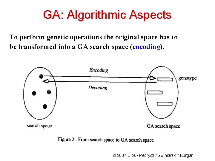
GA: Algorithmic Aspects To perform genetic operations the original space has to be transformed into a GA search space (encoding). © 2007 Cios / Pedrycz / Swiniarski / Kurgan

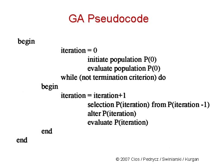
GA Pseudocode © 2007 Cios / Pedrycz / Swiniarski / Kurgan

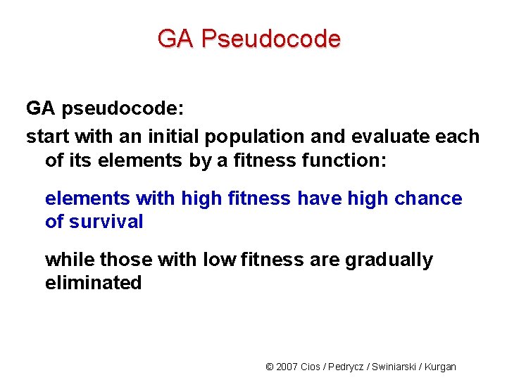
GA Pseudocode GA pseudocode: start with an initial population and evaluate each of its elements by a fitness function: elements with high fitness have high chance of survival while those with low fitness are gradually eliminated © 2007 Cios / Pedrycz / Swiniarski / Kurgan

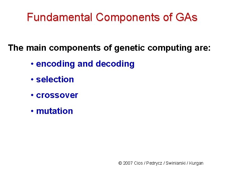
Fundamental Components of GAs The main components of genetic computing are: • encoding and decoding • selection • crossover • mutation © 2007 Cios / Pedrycz / Swiniarski / Kurgan

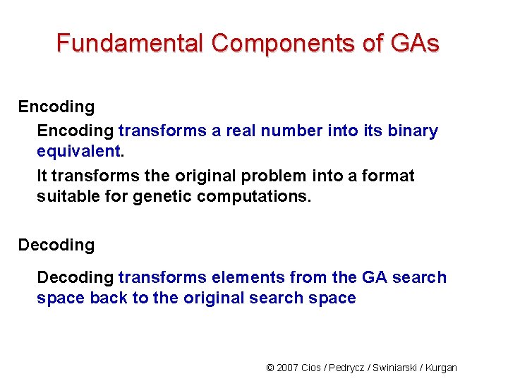
Fundamental Components of GAs Encoding transforms a real number into its binary equivalent. It transforms the original problem into a format suitable for genetic computations. Decoding transforms elements from the GA search space back to the original search space © 2007 Cios / Pedrycz / Swiniarski / Kurgan

Selection Mechanism When a population of chromosomes is established, we must define a way in which the chromosomes are selected for next optimization steps. Selection methods include: • roulette wheel • elitist strategy © 2007 Cios / Pedrycz / Swiniarski / Kurgan

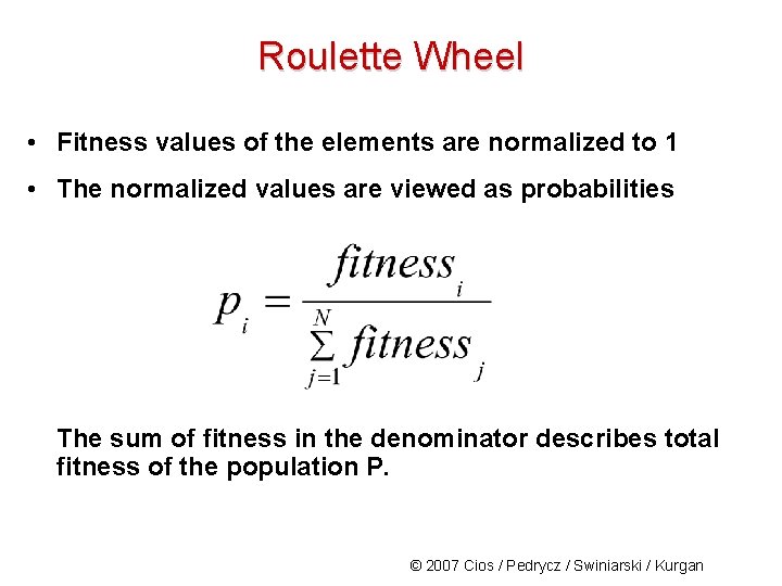
Roulette Wheel • Fitness values of the elements are normalized to 1 • The normalized values are viewed as probabilities The sum of fitness in the denominator describes total fitness of the population P. © 2007 Cios / Pedrycz / Swiniarski / Kurgan

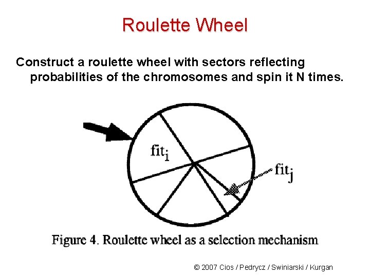
Roulette Wheel Construct a roulette wheel with sectors reflecting probabilities of the chromosomes and spin it N times. © 2007 Cios / Pedrycz / Swiniarski / Kurgan

Elitist Strategy Select the best individuals (strings/chromosomes) in the population and carry them over, without any alteration, to the next population. © 2007 Cios / Pedrycz / Swiniarski / Kurgan

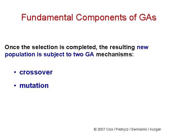
Fundamental Components of GAs Once the selection is completed, the resulting new population is subject to two GA mechanisms: • crossover • mutation © 2007 Cios / Pedrycz / Swiniarski / Kurgan

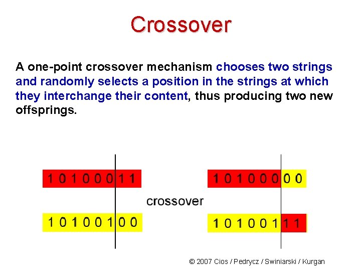
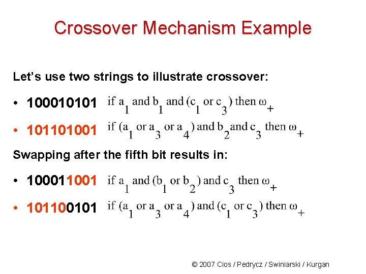
Crossover A one-point crossover mechanism chooses two strings and randomly selects a position in the strings at which they interchange their content, thus producing two new offsprings. © 2007 Cios / Pedrycz / Swiniarski / Kurgan

Crossover • Crossover leads to an increased diversity of the population of strings, as the new individuals with new properties emerge. • The intensity of crossover is characterized in terms of the probability at which the elements of strings are affected; the higher the probability, the more individuals are affected. © 2007 Cios / Pedrycz / Swiniarski / Kurgan

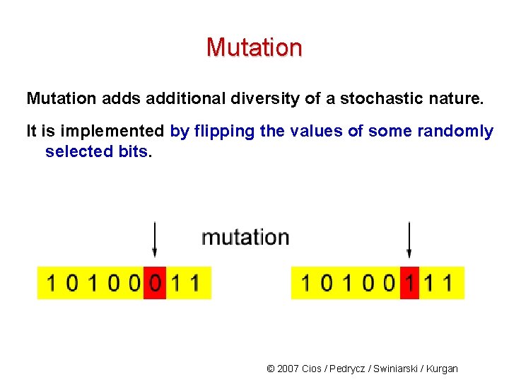
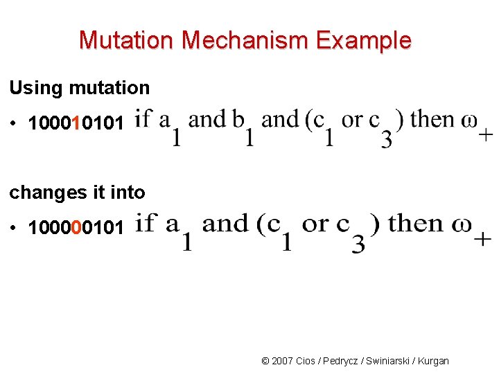
Mutation adds additional diversity of a stochastic nature. It is implemented by flipping the values of some randomly selected bits. © 2007 Cios / Pedrycz / Swiniarski / Kurgan

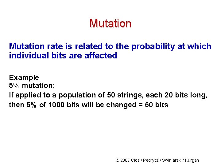
Mutation rate is related to the probability at which individual bits are affected Example 5% mutation: If applied to a population of 50 strings, each 20 bits long, then 5% of 1000 bits will be changed = 50 bits © 2007 Cios / Pedrycz / Swiniarski / Kurgan

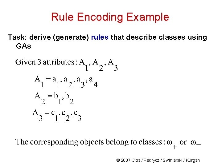
Rule Encoding Example Task: derive (generate) rules that describe classes using GAs © 2007 Cios / Pedrycz / Swiniarski / Kurgan

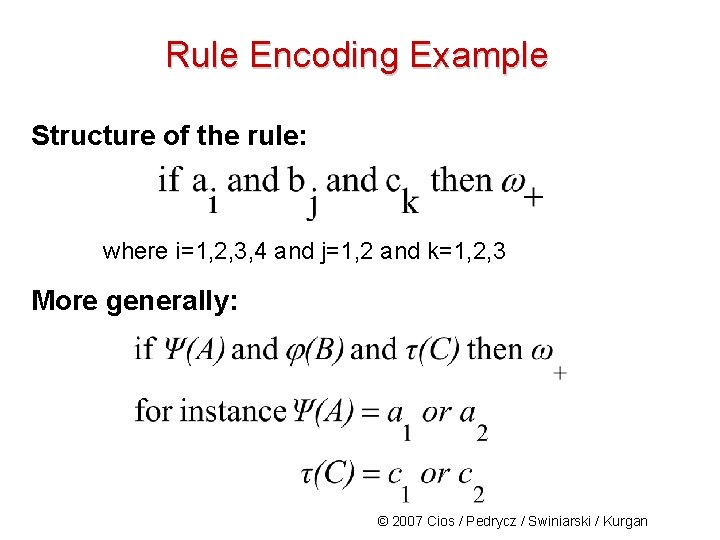
Rule Encoding Example Structure of the rule: where i=1, 2, 3, 4 and j=1, 2 and k=1, 2, 3 More generally: © 2007 Cios / Pedrycz / Swiniarski / Kurgan

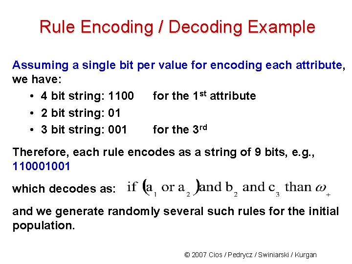
Rule Encoding / Decoding Example Assuming a single bit per value for encoding each attribute, we have: • 4 bit string: 1100 for the 1 st attribute • 2 bit string: 01 • 3 bit string: 001 for the 3 rd Therefore, each rule encodes as a string of 9 bits, e. g. , 110001001 which decodes as: and we generate randomly several such rules for the initial population. © 2007 Cios / Pedrycz / Swiniarski / Kurgan

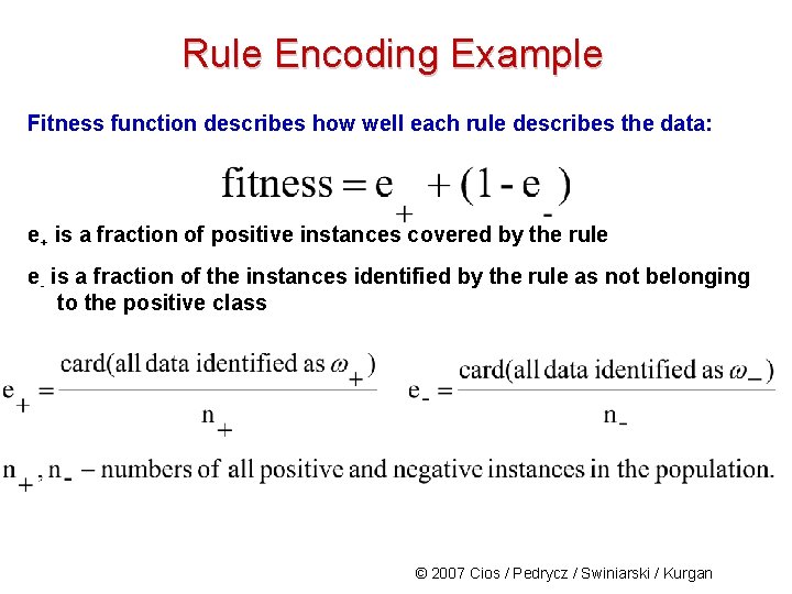
Rule Encoding Example Fitness function describes how well each rule describes the data: e+ is a fraction of positive instances covered by the rule e- is a fraction of the instances identified by the rule as not belonging to the positive class © 2007 Cios / Pedrycz / Swiniarski / Kurgan

Crossover Mechanism Example Let’s use two strings to illustrate crossover: • 100010101 • 101101001 Swapping after the fifth bit results in: • 100011001 • 101100101 © 2007 Cios / Pedrycz / Swiniarski / Kurgan

Mutation Mechanism Example Using mutation • 100010101 changes it into • 100000101 © 2007 Cios / Pedrycz / Swiniarski / Kurgan

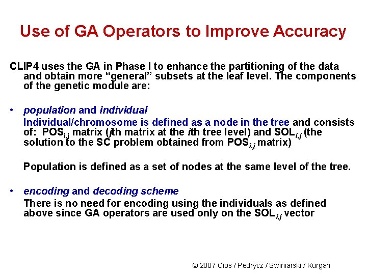
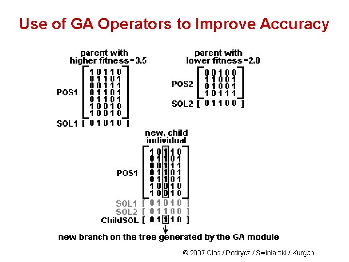
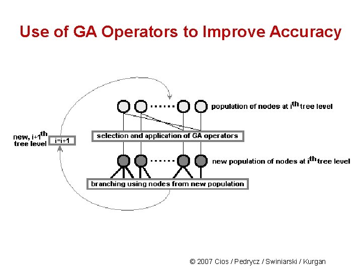
Use of GA Operators to Improve Accuracy CLIP 4 uses the GA in Phase I to enhance the partitioning of the data and obtain more “general” subsets at the leaf level. The components of the genetic module are: • population and individual Individual/chromosome is defined as a node in the tree and consists of: POSi, j matrix (jth matrix at the ith tree level) and SOLi, j (the solution to the SC problem obtained from POSi, j matrix) Population is defined as a set of nodes at the same level of the tree. • encoding and decoding scheme There is no need for encoding using the individuals as defined above since GA operators are used only on the SOLi, j vector © 2007 Cios / Pedrycz / Swiniarski / Kurgan

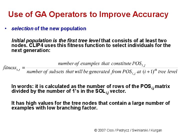
Use of GA Operators to Improve Accuracy • selection of the new population Initial population is the first tree level that consists of at least two nodes. CLIP 4 uses this fitness function to select individuals for the next generation: In words: it is calculated as the number of rows of the POS i, j matrix divided by the number of 1’s in the SOLi, j vector. It has high values for the tree nodes that contain a large number of examples with low branching factor. © 2007 Cios / Pedrycz / Swiniarski / Kurgan

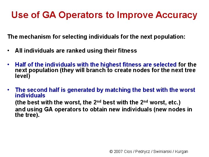
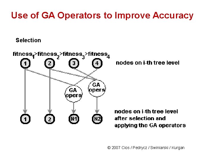
Use of GA Operators to Improve Accuracy The mechanism for selecting individuals for the next population: • All individuals are ranked using their fitness • Half of the individuals with the highest fitness are selected for the next population (they will branch to create nodes for the next tree level) • The second half is generated by matching the best with the worst individuals (the best with the worst, the 2 nd best with the 2 nd worst, etc. ) and using GA operators to obtain new individuals (new nodes in the tree). © 2007 Cios / Pedrycz / Swiniarski / Kurgan

Use of GA Operators to Improve Accuracy Selection © 2007 Cios / Pedrycz / Swiniarski / Kurgan

Use of GA Operators to Improve Accuracy © 2007 Cios / Pedrycz / Swiniarski / Kurgan

Use of GA Operators to Improve Accuracy © 2007 Cios / Pedrycz / Swiniarski / Kurgan

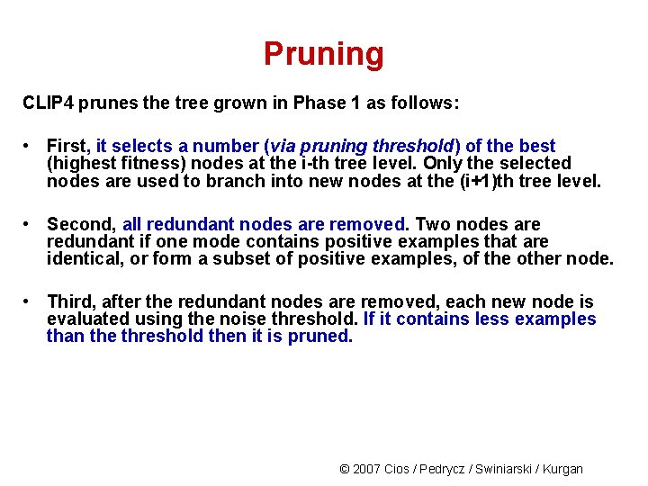
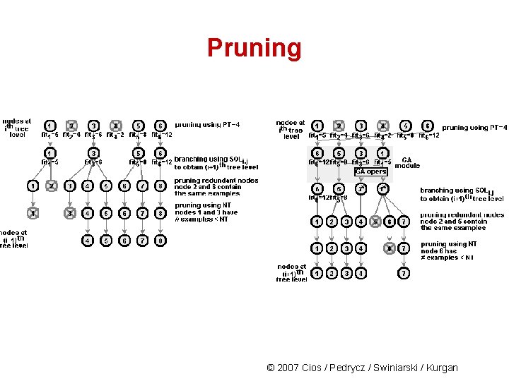
Pruning CLIP 4 prunes the tree grown in Phase 1 as follows: • First, it selects a number (via pruning threshold) of the best (highest fitness) nodes at the i-th tree level. Only the selected nodes are used to branch into new nodes at the (i+1)th tree level. • Second, all redundant nodes are removed. Two nodes are redundant if one mode contains positive examples that are identical, or form a subset of positive examples, of the other node. • Third, after the redundant nodes are removed, each new node is evaluated using the noise threshold. If it contains less examples than the threshold then it is pruned. © 2007 Cios / Pedrycz / Swiniarski / Kurgan

Pruning © 2007 Cios / Pedrycz / Swiniarski / Kurgan

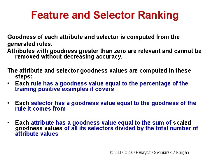
Feature and Selector Ranking Goodness of each attribute and selector is computed from the generated rules. Attributes with goodness greater than zero are relevant and cannot be removed without decreasing accuracy. The attribute and selector goodness values are computed in these steps: • Each rule has a goodness value equal to the percentage of the training positive examples it covers • Each selector has a goodness value equal to the goodness of the rule it comes from • Each attribute has a goodness value equal to the sum of scaled goodness values of all its selectors divided by the total number of attribute values © 2007 Cios / Pedrycz / Swiniarski / Kurgan

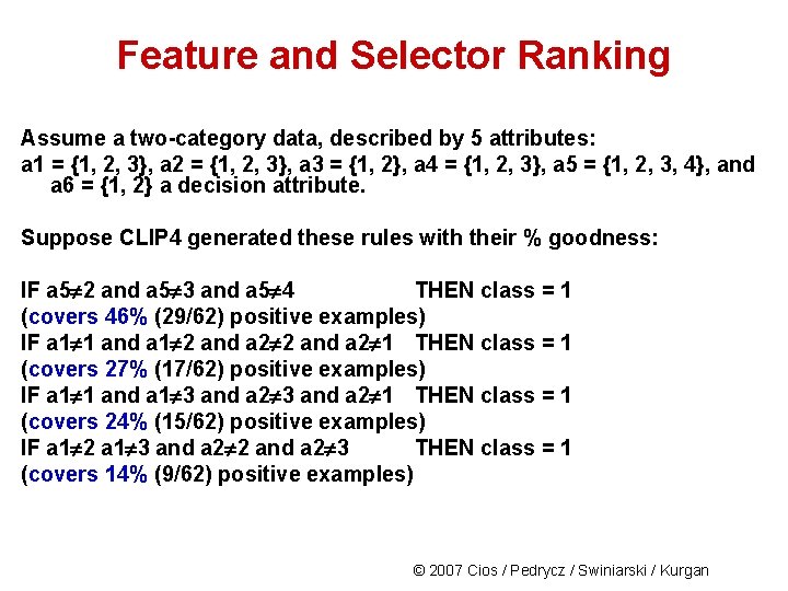
Feature and Selector Ranking Assume a two-category data, described by 5 attributes: a 1 = {1, 2, 3}, a 2 = {1, 2, 3}, a 3 = {1, 2}, a 4 = {1, 2, 3}, a 5 = {1, 2, 3, 4}, and a 6 = {1, 2} a decision attribute. Suppose CLIP 4 generated these rules with their % goodness: IF a 5 2 and a 5 3 and a 5 4 THEN class = 1 (covers 46% (29/62) positive examples) IF a 1 1 and a 1 2 and a 2 1 THEN class = 1 (covers 27% (17/62) positive examples) IF a 1 1 and a 1 3 and a 2 1 THEN class = 1 (covers 24% (15/62) positive examples) IF a 1 2 a 1 3 and a 2 2 and a 2 3 THEN class = 1 (covers 14% (9/62) positive examples) © 2007 Cios / Pedrycz / Swiniarski / Kurgan

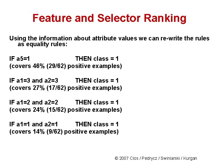
Feature and Selector Ranking Using the information about attribute values we can re-write the rules as equality rules: IF a 5=1 THEN class = 1 (covers 46% (29/62) positive examples) IF a 1=3 and a 2=3 THEN class = 1 (covers 27% (17/62) positive examples) IF a 1=2 and a 2=2 THEN class = 1 (covers 24% (15/62) positive examples) IF a 1=1 and a 2=1 THEN class = 1 (covers 14% (9/62) positive examples) © 2007 Cios / Pedrycz / Swiniarski / Kurgan

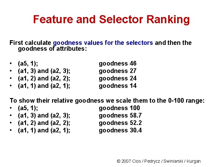
Feature and Selector Ranking First calculate goodness values for the selectors and then the goodness of attributes: • • (a 5, 1); (a 1, 3) and (a 2, 3); (a 1, 2) and (a 2, 2); (a 1, 1) and (a 2, 1); goodness 46 goodness 27 goodness 24 goodness 14 To show their relative goodness we scale them to the 0 -100 range: • (a 5, 1); goodness 100 • (a 1, 3) and (a 2, 3); goodness 58. 7 • (a 1, 2) and (a 2, 2); goodness 52. 2 • (a 1, 1) and (a 2, 1); goodness 30. 4 © 2007 Cios / Pedrycz / Swiniarski / Kurgan

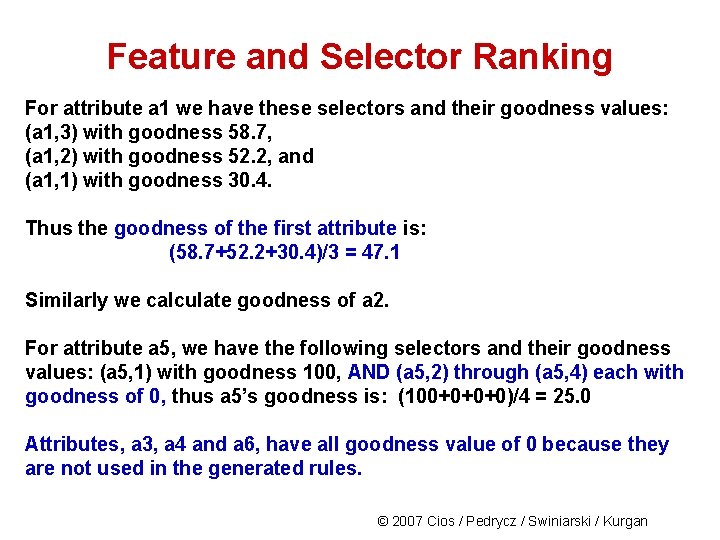
Feature and Selector Ranking For attribute a 1 we have these selectors and their goodness values: (a 1, 3) with goodness 58. 7, (a 1, 2) with goodness 52. 2, and (a 1, 1) with goodness 30. 4. Thus the goodness of the first attribute is: (58. 7+52. 2+30. 4)/3 = 47. 1 Similarly we calculate goodness of a 2. For attribute a 5, we have the following selectors and their goodness values: (a 5, 1) with goodness 100, AND (a 5, 2) through (a 5, 4) each with goodness of 0, thus a 5’s goodness is: (100+0+0+0)/4 = 25. 0 Attributes, a 3, a 4 and a 6, have all goodness value of 0 because they are not used in the generated rules. © 2007 Cios / Pedrycz / Swiniarski / Kurgan

Feature and Selector Ranking The feature and selector ranking performed by CLIP 4 algorithm can be used to: • Select only relevant attributes (and thus discard the irrelevant ones) The user can safely discard all attributes with goodness of 0 and still have the correct (with the same accuracy) model. • Provide additional insight into data properties, e. g. , the selector ranking can help in analyzing data in terms of relevance of the selectors to the classification task. © 2007 Cios / Pedrycz / Swiniarski / Kurgan

References Cios K. J. and Liu N. 1992. Machine learning in generation of a neural network architecture: a Continuous ID 3 approach. IEEE Trans. on Neural Networks, 3(2): 280‑ 291 Cios, K. J. , Pedrycz, W. and Swiniarski, R. 1998. Data Mining Methods for Knowledge Discovery. Kluwer Cios, K. J. and Kurgan, L. 2004. CLIP 4: Hybrid Inductive Machine Learning Algorithm that Generates Inequality Rules. Information Sciences, 163 (1 -3): 37 -83 Kurgan L. , Cios K. J. and Dick S. 2006. Highly Scalable and Robust Rule Learner: Performance Evaluation and Comparison, IEEE Trans. on Systems Man and Cybernetics, Part B, 36(1): 32 -53 Kurgan, L. and Cios, K. J. 2002. CAIM Discretization Algorithm, IEEE Trans. on Knowledge and Data Engineering, 16(2): 145 -153 © 2007 Cios / Pedrycz / Swiniarski / Kurgan