Chapter 12 Statistical Inference Other One Sample Test

Chapter 12 Statistical Inference: Other One. Sample Test Statistics I One-Sample z Test for a Population Proportion, p A. Introduction to z Test for a Population Proportion 1

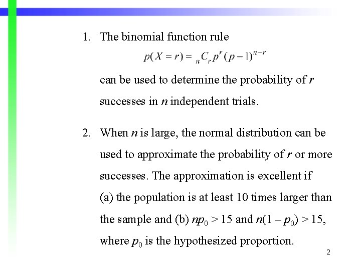
1. The binomial function rule can be used to determine the probability of r successes in n independent trials. 2. When n is large, the normal distribution can be used to approximate the probability of r or more successes. The approximation is excellent if (a) the population is at least 10 times larger than the sample and (b) np 0 > 15 and n(1 – p 0) > 15, where p 0 is the hypothesized proportion. 2

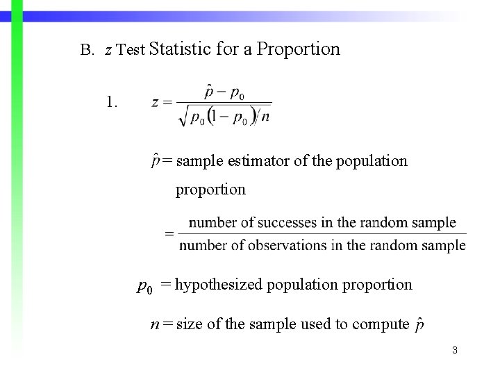
B. z Test Statistic for a Proportion 1. = sample estimator of the population proportion p 0 = hypothesized population proportion n = size of the sample used to compute 3

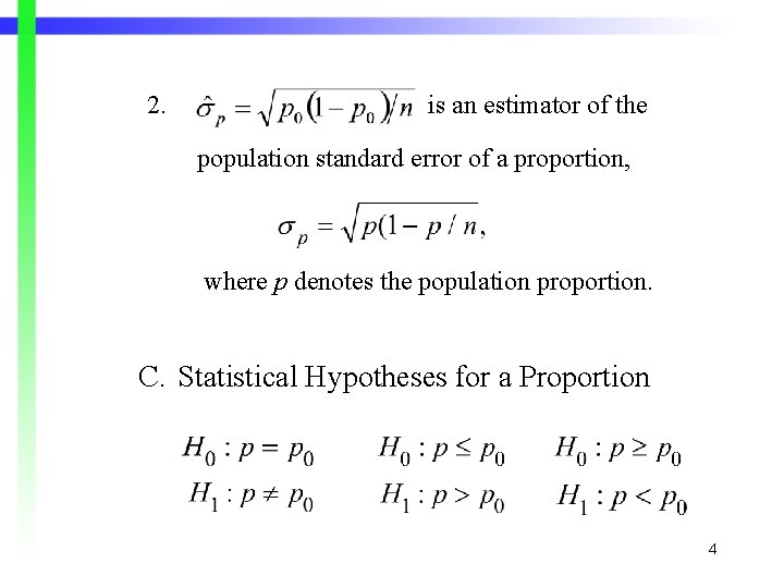
2. is an estimator of the population standard error of a proportion, where p denotes the population proportion. C. Statistical Hypotheses for a Proportion 4

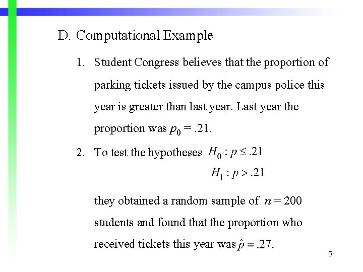
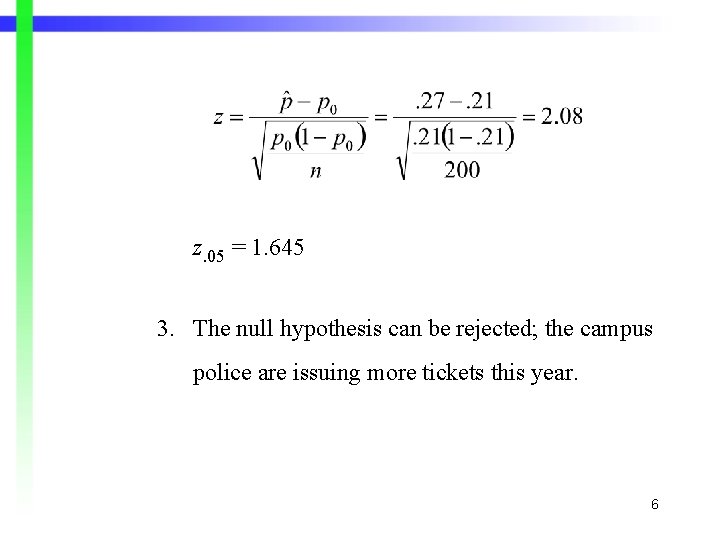
D. Computational Example 1. Student Congress believes that the proportion of parking tickets issued by the campus police this year is greater than last year. Last year the proportion was p 0 =. 21. 2. To test the hypotheses they obtained a random sample of n = 200 students and found that the proportion who received tickets this year was 5

z. 05 = 1. 645 3. The null hypothesis can be rejected; the campus police are issuing more tickets this year. 6

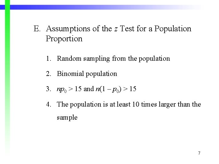
E. Assumptions of the z Test for a Population Proportion 1. Random sampling from the population 2. Binomial population 3. np 0 > 15 and n(1 – p 0) > 15 4. The population is at least 10 times larger than the sample 7

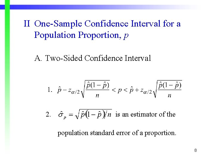
II One-Sample Confidence Interval for a Population Proportion, p A. Two-Sided Confidence Interval 2. is an estimator of the population standard error of a proportion. 8

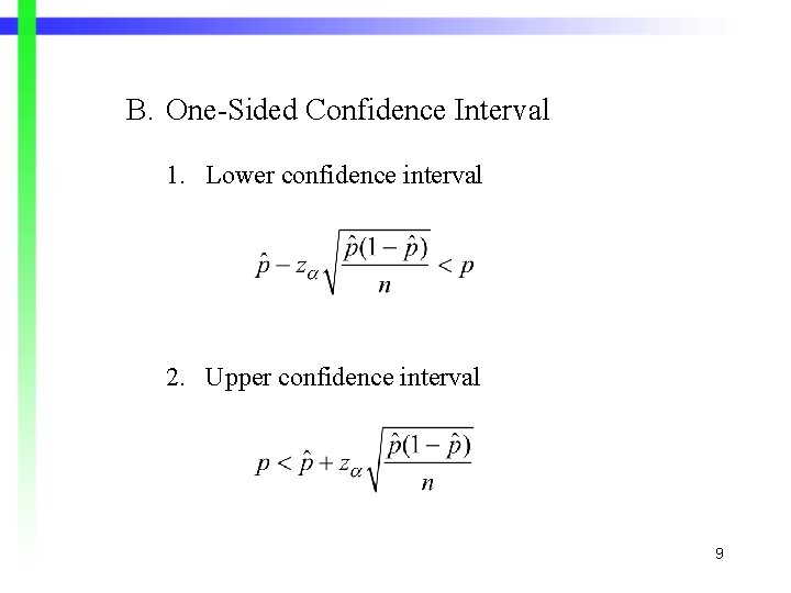
B. One-Sided Confidence Interval 1. Lower confidence interval 2. Upper confidence interval 9

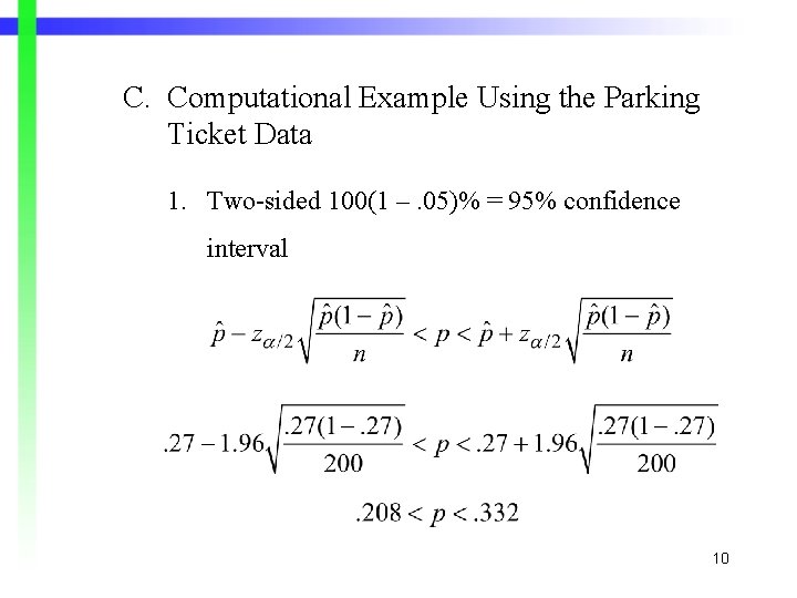
C. Computational Example Using the Parking Ticket Data 1. Two-sided 100(1 –. 05)% = 95% confidence interval 10

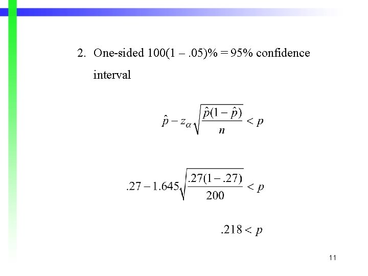
2. One-sided 100(1 –. 05)% = 95% confidence interval 11

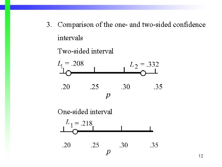
3. Comparison of the one- and two-sided confidence intervals Two-sided interval One-sided interval 12

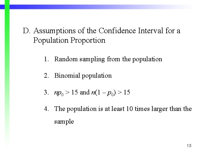
D. Assumptions of the Confidence Interval for a Population Proportion 1. Random sampling from the population 2. Binomial population 3. np 0 > 15 and n(1 – p 0) > 15 4. The population is at least 10 times larger than the sample 13

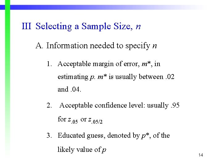
III Selecting a Sample Size, n A. Information needed to specify n 1. Acceptable margin of error, m*, in estimating p. m* is usually between. 02 and. 04. 2. Acceptable confidence level: usually. 95 for z. 05/2 3. Educated guess, denoted by p*, of the likely value of p 14

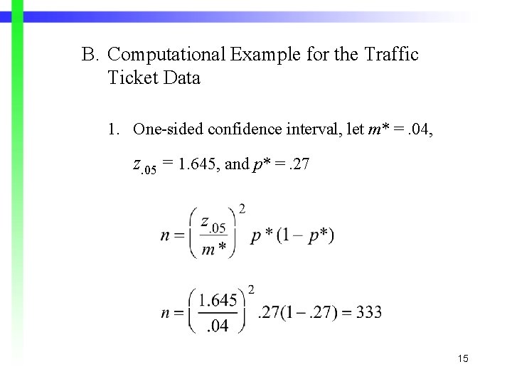
B. Computational Example for the Traffic Ticket Data 1. One-sided confidence interval, let m* =. 04, z. 05 = 1. 645, and p* =. 27 15

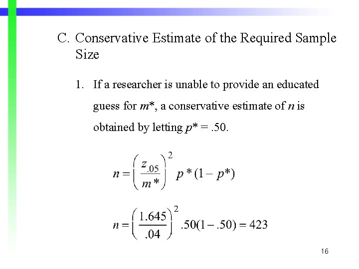
C. Conservative Estimate of the Required Sample Size 1. If a researcher is unable to provide an educated guess for m*, a conservative estimate of n is obtained by letting p* =. 50. 16

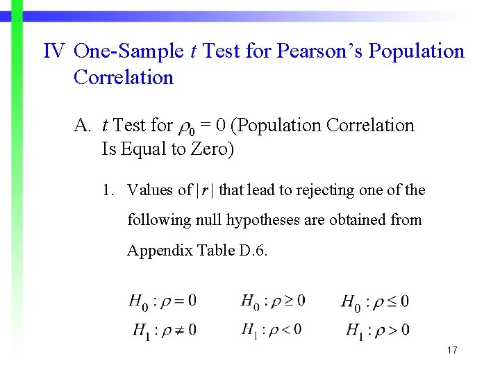
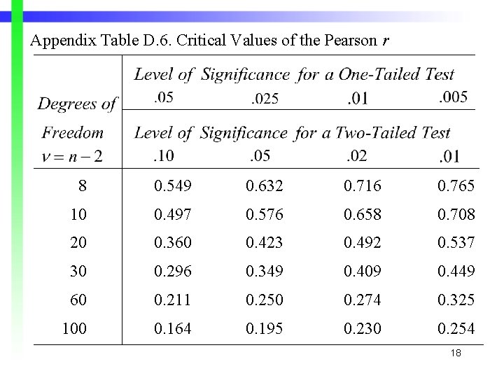
IV One-Sample t Test for Pearson’s Population Correlation A. t Test for 0 = 0 (Population Correlation Is Equal to Zero) 1. Values of | r | that lead to rejecting one of the following null hypotheses are obtained from Appendix Table D. 6. 17

Appendix Table D. 6. Critical Values of the Pearson r 8 0. 549 0. 632 0. 716 0. 765 10 0. 497 0. 576 0. 658 0. 708 20 0. 360 0. 423 0. 492 0. 537 30 0. 296 0. 349 0. 409 0. 449 60 0. 211 0. 250 0. 274 0. 325 100 0. 164 0. 195 0. 230 0. 254 18

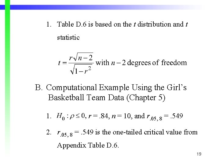
1. Table D. 6 is based on the t distribution and t statistic B. Computational Example Using the Girl’s Basketball Team Data (Chapter 5) 1. r =. 84, n = 10, and r. 05, 8 =. 549 2. r. 05, 8 =. 549 is the one-tailed critical value from Appendix Table D. 6. 19

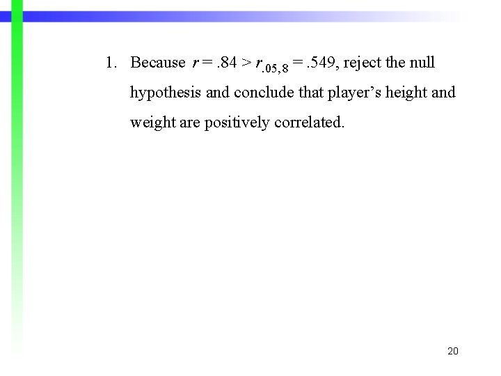
1. Because r =. 84 > r. 05, 8 =. 549, reject the null hypothesis and conclude that player’s height and weight are positively correlated. 20

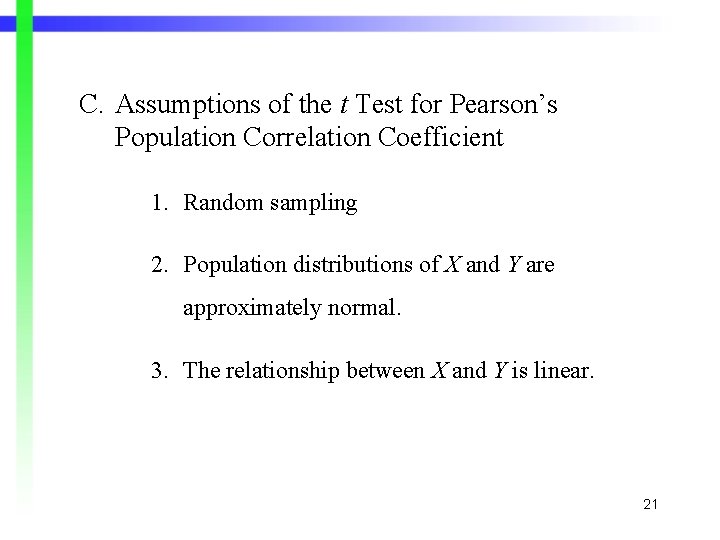
C. Assumptions of the t Test for Pearson’s Population Correlation Coefficient 1. Random sampling 2. Population distributions of X and Y are approximately normal. 3. The relationship between X and Y is linear. 21

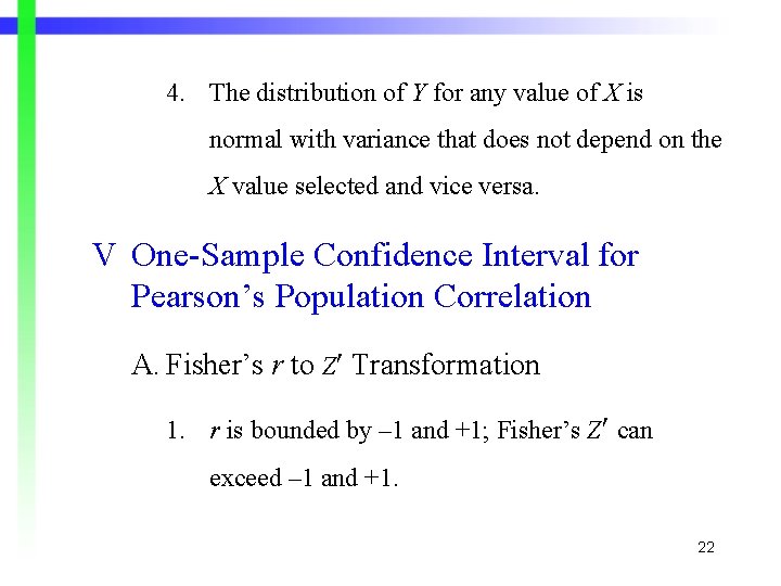
4. The distribution of Y for any value of X is normal with variance that does not depend on the X value selected and vice versa. V One-Sample Confidence Interval for Pearson’s Population Correlation A. Fisher’s r to Z Transformation 1. r is bounded by – 1 and +1; Fisher’s Z can exceed – 1 and +1. 22

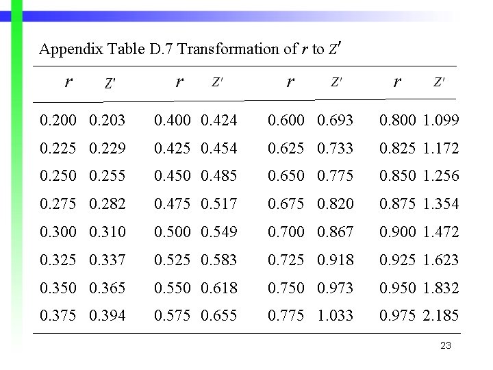
Appendix Table D. 7 Transformation of r to Z 0. 200 0. 203 0. 400 0. 424 0. 600 0. 693 0. 800 1. 099 0. 225 0. 229 0. 425 0. 454 0. 625 0. 733 0. 825 1. 172 0. 250 0. 255 0. 450 0. 485 0. 650 0. 775 0. 850 1. 256 0. 275 0. 282 0. 475 0. 517 0. 675 0. 820 0. 875 1. 354 0. 300 0. 310 0. 500 0. 549 0. 700 0. 867 0. 900 1. 472 0. 325 0. 337 0. 525 0. 583 0. 725 0. 918 0. 925 1. 623 0. 350 0. 365 0. 550 0. 618 0. 750 0. 973 0. 950 1. 832 0. 375 0. 394 0. 575 0. 655 0. 775 1. 033 0. 975 2. 185 23

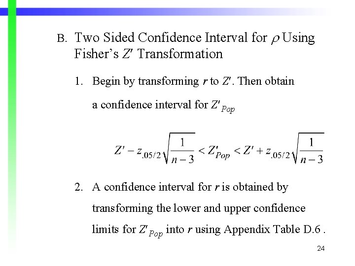
B. Two Sided Confidence Interval for Using Fisher’s Z Transformation 1. Begin by transforming r to Z. Then obtain a confidence interval for Z Pop 2. A confidence interval for r is obtained by transforming the lower and upper confidence limits for Z Pop into r using Appendix Table D. 6. 24

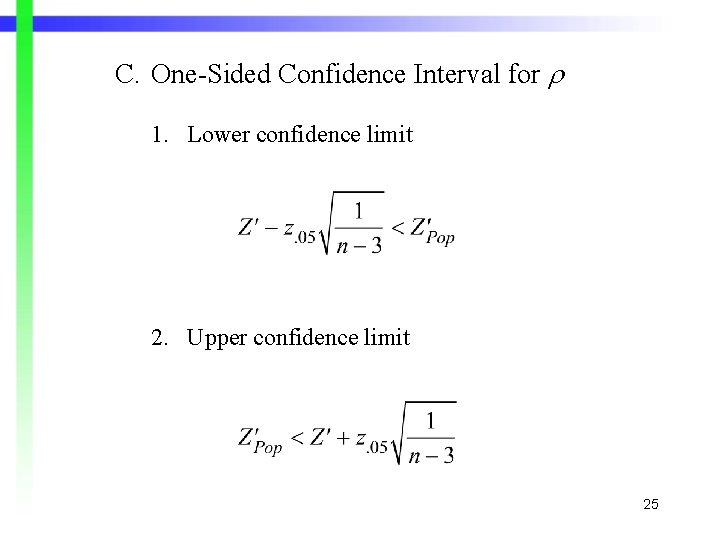
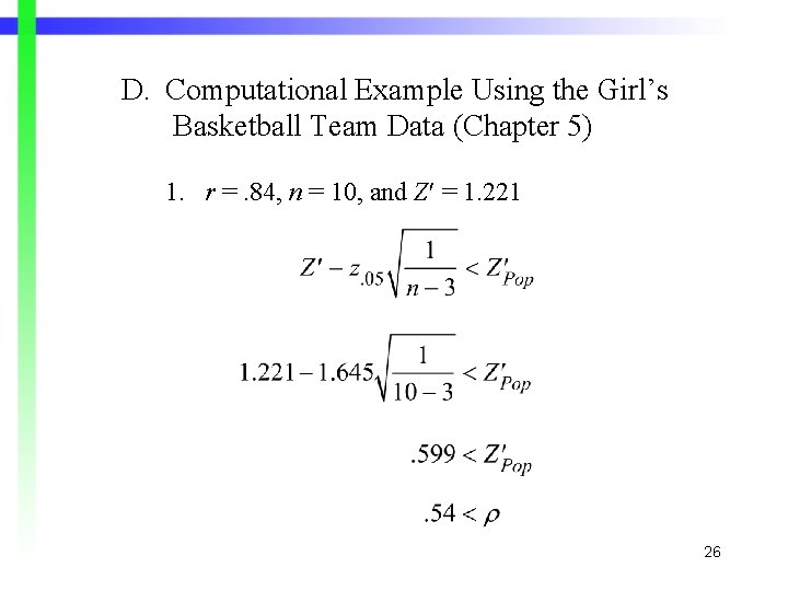
C. One-Sided Confidence Interval for 1. Lower confidence limit 2. Upper confidence limit 25

D. Computational Example Using the Girl’s Basketball Team Data (Chapter 5) 1. r =. 84, n = 10, and Z = 1. 221 26

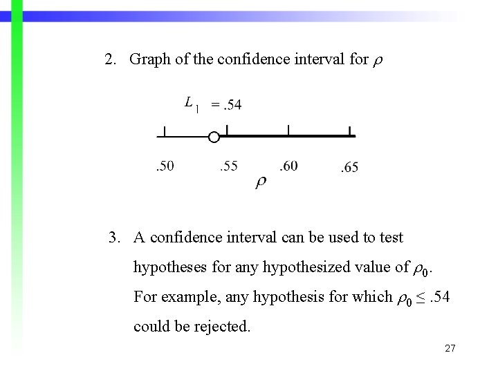
2. Graph of the confidence interval for 3. A confidence interval can be used to test hypotheses for any hypothesized value of 0. For example, any hypothesis for which 0 ≤. 54 could be rejected. 27

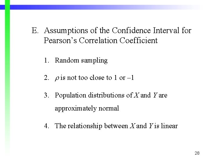
E. Assumptions of the Confidence Interval for Pearson’s Correlation Coefficient 1. Random sampling 2. is not too close to 1 or – 1 3. Population distributions of X and Y are approximately normal 4. The relationship between X and Y is linear 28

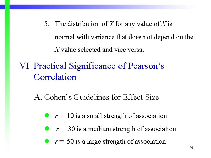
5. The distribution of Y for any value of X is normal with variance that does not depend on the X value selected and vice versa. VI Practical Significance of Pearson’s Correlation A. Cohen’s Guidelines for Effect Size r =. 10 is a small strength of association r =. 30 is a medium strength of association r =. 50 is a large strength of association 29