Chapter 12 Monte Carlo Simulation and Risk Analysis

Chapter 12 Monte Carlo Simulation and Risk Analysis

Model Uncertainty and Risk Analysis Many situations dictate that randomness be explicitly incorporated into our models. This is usually done by specifying probability distributions for the appropriate uncontrollable inputs. ◦ Such models are called stochastic, or probabilistic. Risk is the likelihood of an undesirable outcome. It can be assessed by evaluating the probability that the outcome will occur along with the severity of the outcome. Risk analysis seeks to examine the impact of uncertain inputs on various outputs.

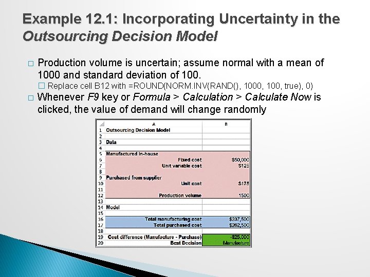
Example 12. 1: Incorporating Uncertainty in the Outsourcing Decision Model � Production volume is uncertain; assume normal with a mean of 1000 and standard deviation of 100. � Replace cell B 12 with =ROUND(NORM. INV(RAND(), 1000, 100, true), 0) � Whenever F 9 key or Formula > Calculation > Calculate Now is clicked, the value of demand will change randomly

Monte Carlo Simulation Monte Carlo simulation is the process of generating random values for uncertain inputs in a model, computing the output variables of interest, and repeating this process for many trials to understand the distribution of the output results. Monte Carlo simulation can easily be accomplished on a spreadsheet using a data table.

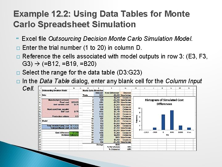
Example 12. 2: Using Data Tables for Monte Carlo Spreadsheet Simulation Excel file Outsourcing Decision Monte Carlo Simulation Model. � Enter the trial number (1 to 20) in column D. � Reference the cells associated with model outputs in row 3: (E 3, F 3, G 3) (=B 12, =B 19, =B 20) � Select the range for the data table (D 3: G 23) � In the Data Table dialog, enter any blank cell for the Column Input Cell.

Monte Carlo Simulation Using Analytic Solver Platform 1. Develop a spreadsheet model. 2. Determine probability distributions for uncertain input variables. 3. Identify output variables you want to predict. 4. Choose the number of trials for the simulation. 5. Run the simulation. 6. Interpret the results.

Defining Uncertain Model Inputs For many decision models, empirical data may be available, either in historical records or collected through special efforts. In other situations, historical data are not available, and we can draw upon the properties of common probability distributions to help choose a representative distribution that has the shape that would most reasonably represent the analyst’s understanding about the uncertain variable. Uniform or triangular distributions are often used in the absence of data. In Analytic Solver Platform, use custom Excel functions or the Distributions button in the ribbon.

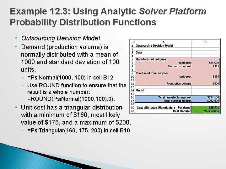
Example 12. 3: Using Analytic Solver Platform Probability Distribution Functions Outsourcing Decision Model Demand (production volume) is normally distributed with a mean of 1000 and standard deviation of 100 units. ◦ =Psi. Normal(1000, 100) in cell B 12 ◦ Use ROUND function to ensure that the result is a whole number: =ROUND(Psi. Normal(1000, 100), 0). Unit cost has a triangular distribution with a minimum of $160, most likely value of $175, and a maximum of $200. ◦ =Psi. Triangular(160, 175, 200) in cell B 10.

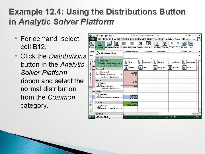
Example 12. 4: Using the Distributions Button in Analytic Solver Platform For demand, select cell B 12. Click the Distributions button in the Analytic Solver Platform ribbon and select the normal distribution from the Common category.

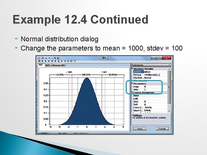
Example 12. 4 Continued Normal distribution dialog Change the parameters to mean = 1000, stdev = 100

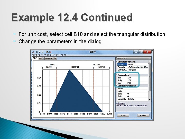
Example 12. 4 Continued For unit cost, select cell B 10 and select the triangular distribution Change the parameters in the dialog

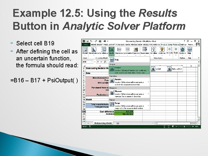
Defining Output Cells To define a cell you wish to predict and create a distribution of output values from your model, first select it, and then click on the Results button in the Simulation Model group in the Analytic Solver Platform ribbon. Choose the Output option and then In Cell. ◦ Analytic Solver Platform calls output cells uncertain function cells. ◦ Uncertain function cells must be numeric. Analytic Solver Platform adds the function Psi. Output( ) to uncertain function cell formulas. ◦ You may also add +Psi. Output( ) to any output cells manually

Example 12. 5: Using the Results Button in Analytic Solver Platform Select cell B 19 After defining the cell as an uncertain function, the formula should read: =B 16 – B 17 + Psi. Output( )

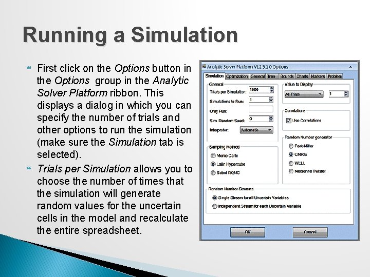
Running a Simulation First click on the Options button in the Options group in the Analytic Solver Platform ribbon. This displays a dialog in which you can specify the number of trials and other options to run the simulation (make sure the Simulation tab is selected). Trials per Simulation allows you to choose the number of times that the simulation will generate random values for the uncertain cells in the model and recalculate the entire spreadsheet.

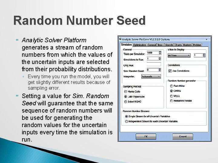
Random Number Seed Analytic Solver Platform generates a stream of random numbers from which the values of the uncertain inputs are selected from their probability distributions. ◦ Every time you run the model, you will get slightly different results because of sampling error. Setting a value for Sim. Random Seed will guarantee that the same sequence of random numbers will be used for generating the random values for the uncertain inputs every time the simulation is run.

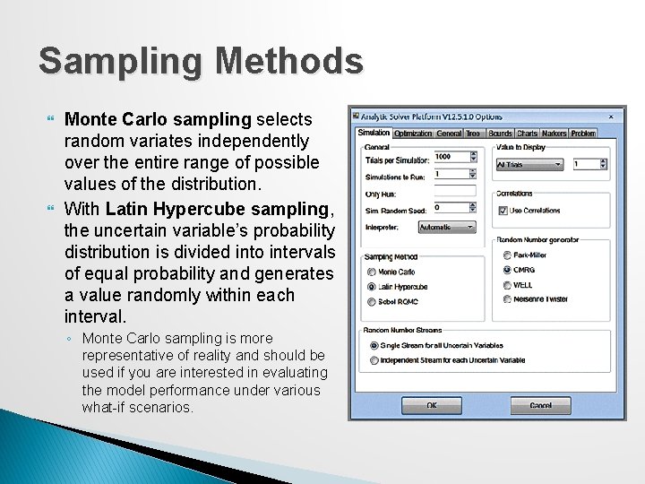
Sampling Methods Monte Carlo sampling selects random variates independently over the entire range of possible values of the distribution. With Latin Hypercube sampling, the uncertain variable’s probability distribution is divided into intervals of equal probability and generates a value randomly within each interval. ◦ Monte Carlo sampling is more representative of reality and should be used if you are interested in evaluating the model performance under various what-if scenarios.

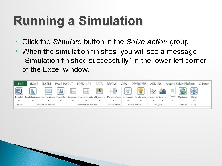
Running a Simulation Click the Simulate button in the Solve Action group. When the simulation finishes, you will see a message “Simulation finished successfully” in the lower-left corner of the Excel window.

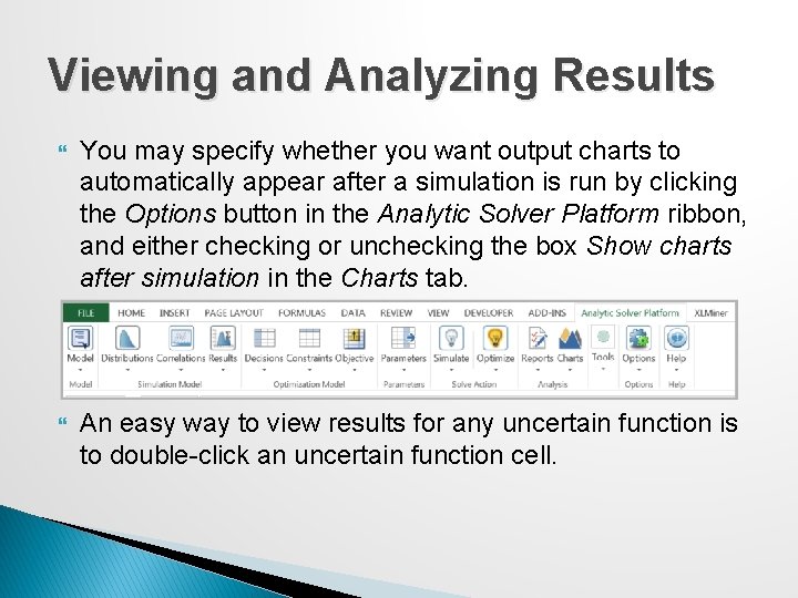
Viewing and Analyzing Results You may specify whether you want output charts to automatically appear after a simulation is run by clicking the Options button in the Analytic Solver Platform ribbon, and either checking or unchecking the box Show charts after simulation in the Charts tab. An easy way to view results for any uncertain function is to double-click an uncertain function cell.

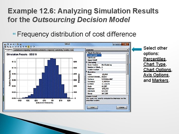
Example 12. 6: Analyzing Simulation Results for the Outsourcing Decision Model Frequency distribution of cost difference Select other options: Percentiles, Chart Type, Chart Options, Axis Options, and Markers.

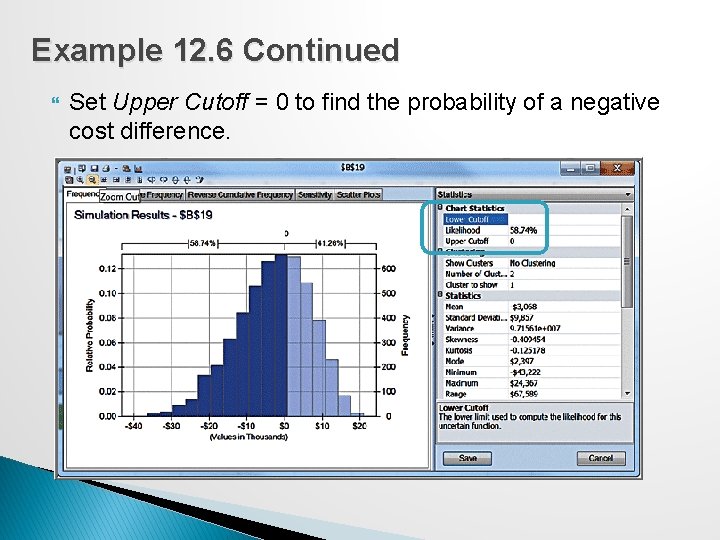
Example 12. 6 Continued Set Upper Cutoff = 0 to find the probability of a negative cost difference.

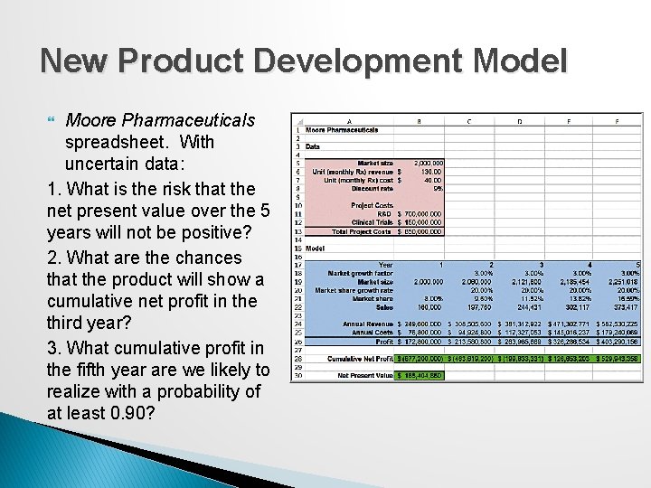
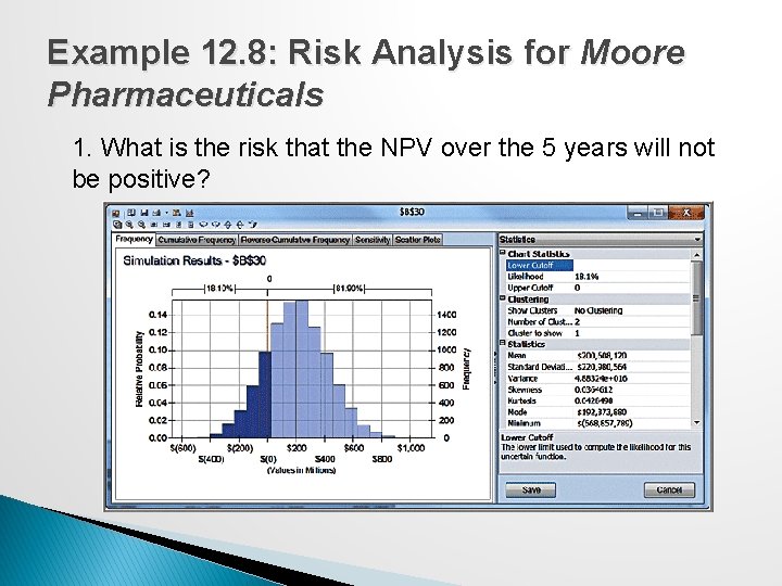
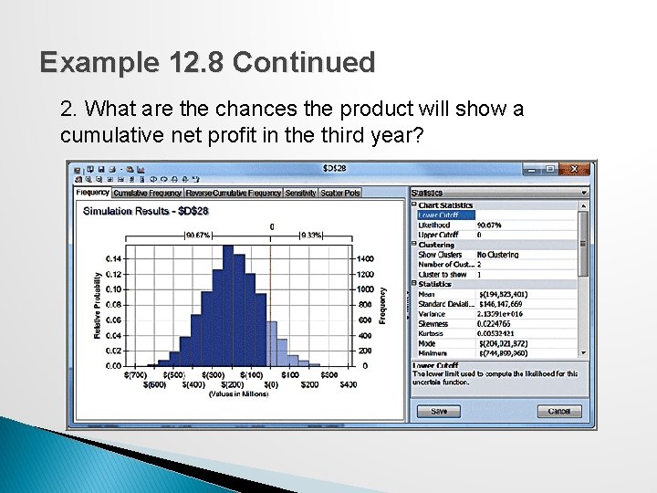
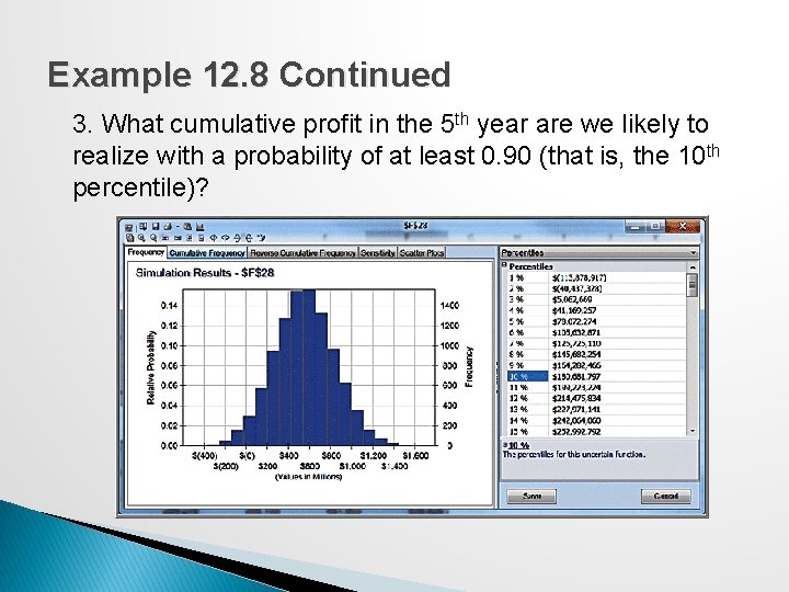
New Product Development Model Moore Pharmaceuticals spreadsheet. With uncertain data: 1. What is the risk that the net present value over the 5 years will not be positive? 2. What are the chances that the product will show a cumulative net profit in the third year? 3. What cumulative profit in the fifth year are we likely to realize with a probability of at least 0. 90?

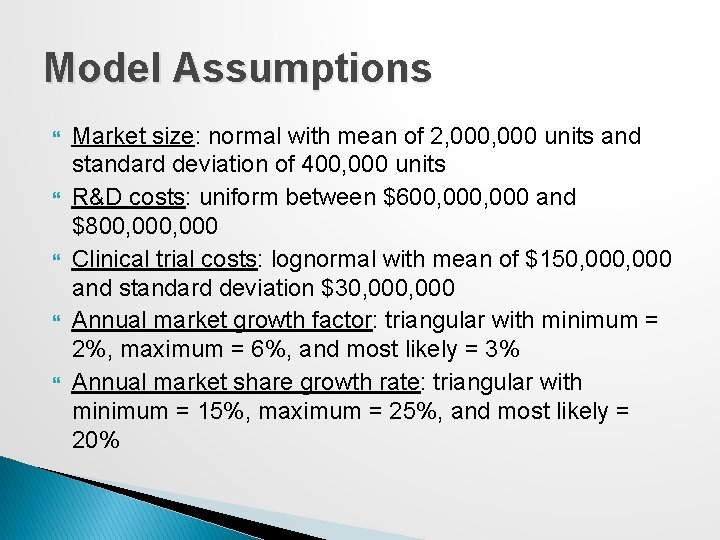
Model Assumptions Market size: normal with mean of 2, 000 units and standard deviation of 400, 000 units R&D costs: uniform between $600, 000 and $800, 000 Clinical trial costs: lognormal with mean of $150, 000 and standard deviation $30, 000 Annual market growth factor: triangular with minimum = 2%, maximum = 6%, and most likely = 3% Annual market share growth rate: triangular with minimum = 15%, maximum = 25%, and most likely = 20%

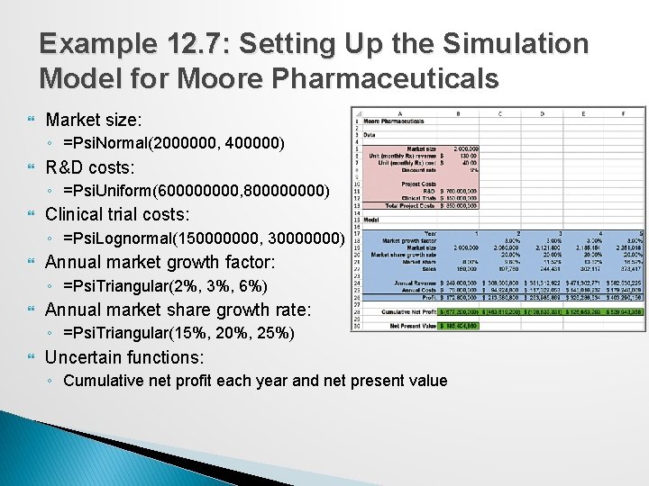
Example 12. 7: Setting Up the Simulation Model for Moore Pharmaceuticals Market size: ◦ =Psi. Normal(2000000, 400000) R&D costs: ◦ =Psi. Uniform(60000, 80000) Clinical trial costs: ◦ =Psi. Lognormal(150000000, 30000000) Annual market growth factor: ◦ =Psi. Triangular(2%, 3%, 6%) Annual market share growth rate: ◦ =Psi. Triangular(15%, 20%, 25%) Uncertain functions: ◦ Cumulative net profit each year and net present value

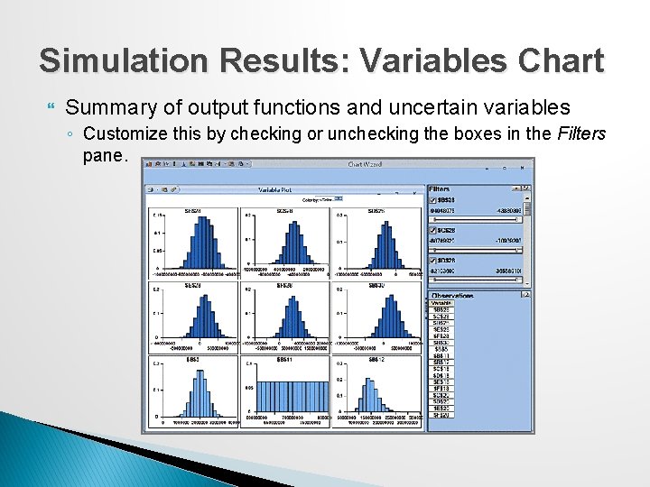
Simulation Results: Variables Chart Summary of output functions and uncertain variables ◦ Customize this by checking or unchecking the boxes in the Filters pane.

Example 12. 8: Risk Analysis for Moore Pharmaceuticals 1. What is the risk that the NPV over the 5 years will not be positive?

Example 12. 8 Continued 2. What are the chances the product will show a cumulative net profit in the third year?

Example 12. 8 Continued 3. What cumulative profit in the 5 th year are we likely to realize with a probability of at least 0. 90 (that is, the 10 th percentile)?

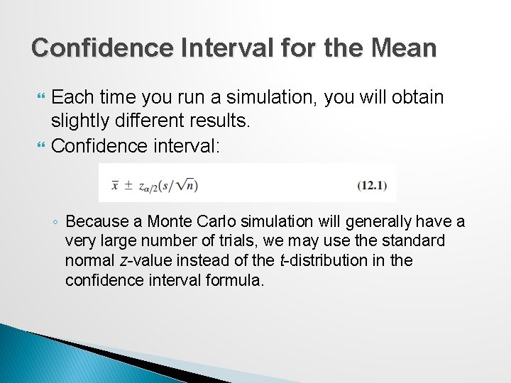
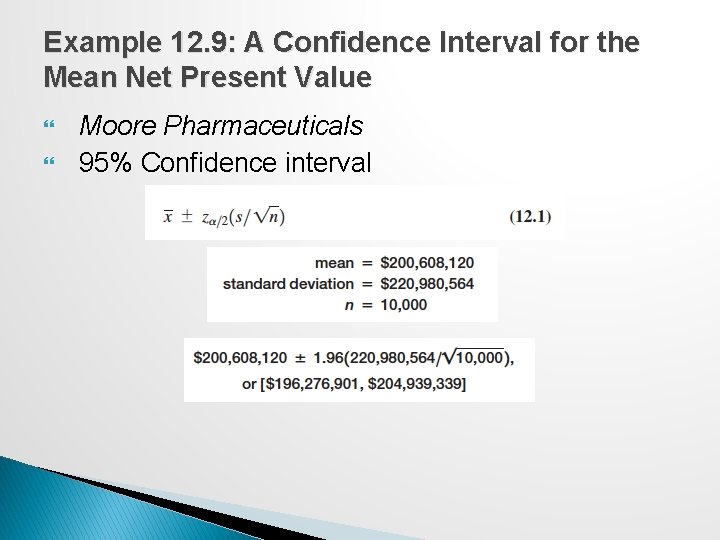
Confidence Interval for the Mean Each time you run a simulation, you will obtain slightly different results. Confidence interval: ◦ Because a Monte Carlo simulation will generally have a very large number of trials, we may use the standard normal z-value instead of the t-distribution in the confidence interval formula.

Example 12. 9: A Confidence Interval for the Mean Net Present Value Moore Pharmaceuticals 95% Confidence interval

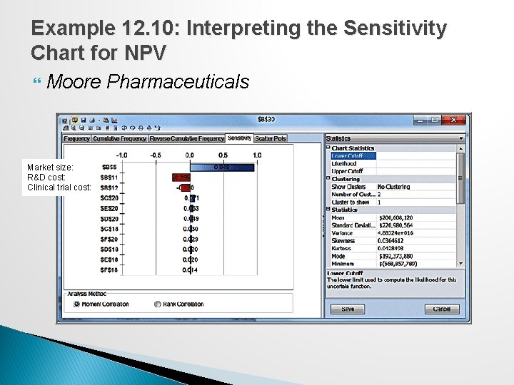
Sensitivity Chart A sensitivity chart allows you to determine the influence that each uncertain model input has individually on an output variable based on its correlation with the output variable. ◦ Displays rankings of uncertain variables according to their impact on an output cell. Benefits: ◦ It tells which uncertain variables influence output variables the most and which would benefit from better estimates. ◦ It tells which uncertain variables influence output variables the least and can be ignored or discarded altogether. ◦ By providing understanding of how the uncertain variables affect your model, it allows you to develop more realistic spreadsheet models and improve the accuracy of your results. Click on the Sensitivity tab in the Simulation Results window.

Example 12. 10: Interpreting the Sensitivity Chart for NPV Moore Pharmaceuticals Market size: R&D cost: Clinical trial cost:

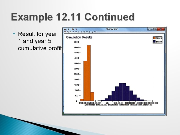
Overlay Charts If a simulation has multiple related forecasts, an overlay chart superimposes the frequency distributions from selected forecasts on one chart in order to compare differences and similarities that might not be apparent.

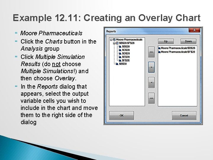
Example 12. 11: Creating an Overlay Chart Moore Pharmaceuticals Click the Charts button in the Analysis group Click Multiple Simulation Results (do not choose Multiple Simulations!) and then choose Overlay. In the Reports dialog that appears, select the output variable cells you wish to include in the chart and move them to the right side of the dialog

Example 12. 11 Continued Result for year 1 and year 5 cumulative profit

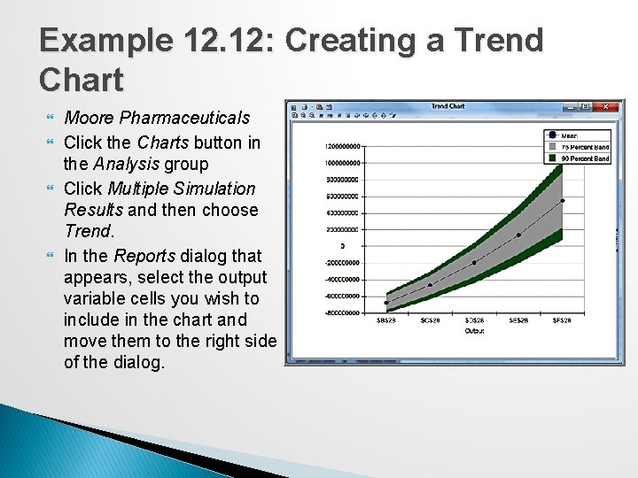
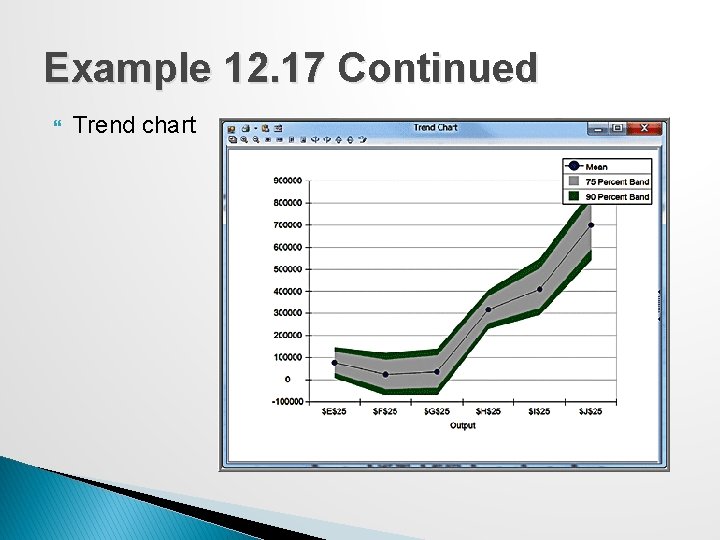
Trend Charts If a simulation has multiple output variables that are related to one another (such as over time), you can view the distributions of all output variables on a single chart, called a trend chart. ◦ A trend chart shows the mean values as well as 75% and 90% bands (probability intervals) around the mean.

Example 12. 12: Creating a Trend Chart Moore Pharmaceuticals Click the Charts button in the Analysis group Click Multiple Simulation Results and then choose Trend. In the Reports dialog that appears, select the output variable cells you wish to include in the chart and move them to the right side of the dialog.

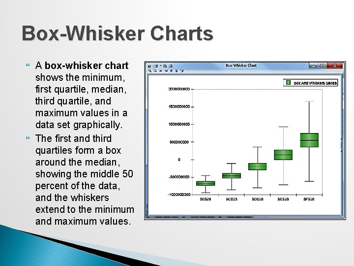
Box-Whisker Charts A box-whisker chart shows the minimum, first quartile, median, third quartile, and maximum values in a data set graphically. The first and third quartiles form a box around the median, showing the middle 50 percent of the data, and the whiskers extend to the minimum and maximum values.

Simulation Reports Analytic Solver Platform creates reports in the form of Excel worksheets that summarize a simulation. Click the Reports button in the Analysis group in the ribbon, and choose Simulation from the options that appear. The report summarizes basic statistical information about the model, simulation options, uncertain variables, and output variables,

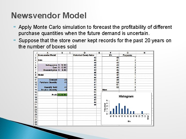
Newsvendor Model Apply Monte Carlo simulation to forecast the profitability of different purchase quantities when the future demand is uncertain. Suppose that the store owner kept records for the past 20 years on the number of boxes sold

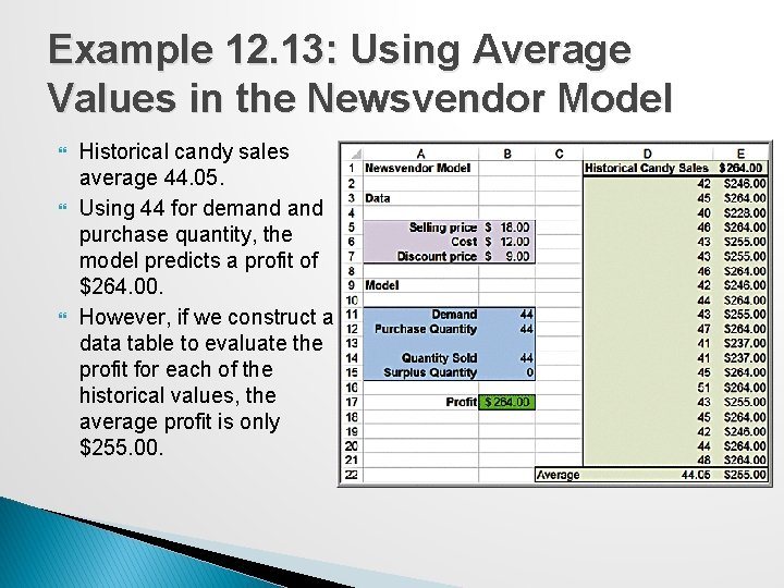
Example 12. 13: Using Average Values in the Newsvendor Model Historical candy sales average 44. 05. Using 44 for demand purchase quantity, the model predicts a profit of $264. 00. However, if we construct a data table to evaluate the profit for each of the historical values, the average profit is only $255. 00.

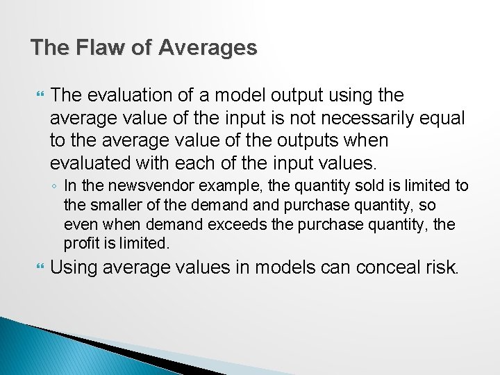
The Flaw of Averages The evaluation of a model output using the average value of the input is not necessarily equal to the average value of the outputs when evaluated with each of the input values. ◦ In the newsvendor example, the quantity sold is limited to the smaller of the demand purchase quantity, so even when demand exceeds the purchase quantity, the profit is limited. Using average values in models can conceal risk.

Monte Carlo Simulation Using Historical Data We can perform a Monte Carlo simulation by resampling from the historical sales distribution— that is, by selecting a value randomly from the historical data.

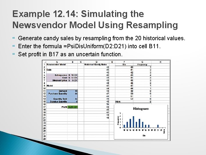
Example 12. 14: Simulating the Newsvendor Model Using Resampling Generate candy sales by resampling from the 20 historical values. Enter the formula =Psi. Dis. Uniform(D 2: D 21) into cell B 11. Set profit in B 17 as an uncertain function.

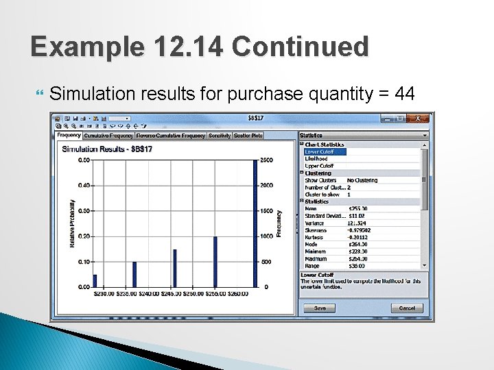
Example 12. 14 Continued Simulation results for purchase quantity = 44

Monte Carlo Simulation Using a Fitted Distribution Sampling from empirical data has some drawbacks. ◦ The empirical data may not adequately represent the true underlying population because of sampling error. ◦ Using an empirical distribution precludes sampling values outside the range of the actual data. It is usually advisable to fit a distribution using the techniques described in Chapter 5 and use it for the uncertain variable.

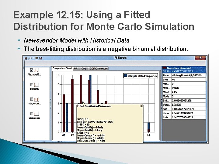
Example 12. 15: Using a Fitted Distribution for Monte Carlo Simulation Newsvendor Model with Historical Data The best-fitting distribution is a negative binomial distribution.

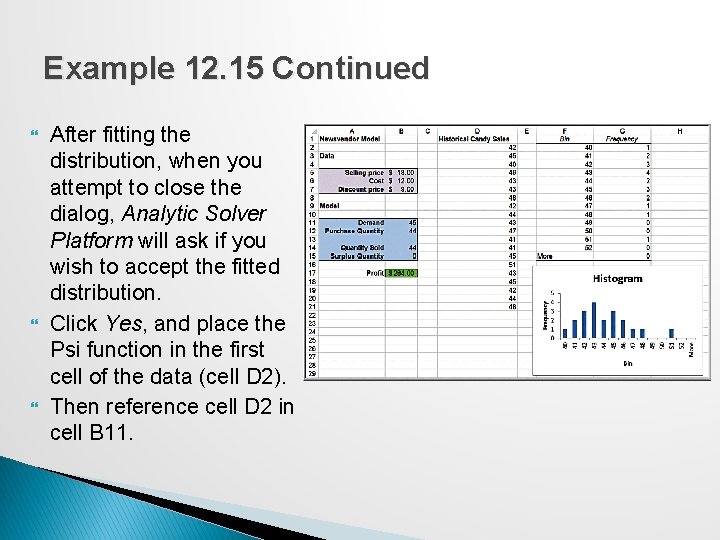
Example 12. 15 Continued After fitting the distribution, when you attempt to close the dialog, Analytic Solver Platform will ask if you wish to accept the fitted distribution. Click Yes, and place the Psi function in the first cell of the data (cell D 2). Then reference cell D 2 in cell B 11.

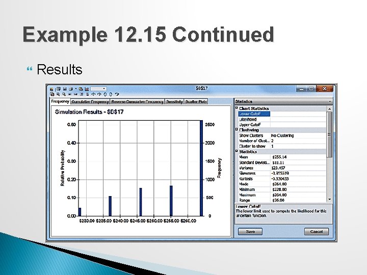
Example 12. 15 Continued Results

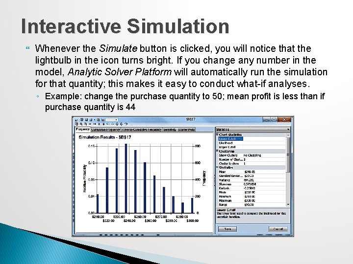
Interactive Simulation Whenever the Simulate button is clicked, you will notice that the lightbulb in the icon turns bright. If you change any number in the model, Analytic Solver Platform will automatically run the simulation for that quantity; this makes it easy to conduct what-if analyses. ◦ Example: change the purchase quantity to 50; mean profit is less than if purchase quantity is 44

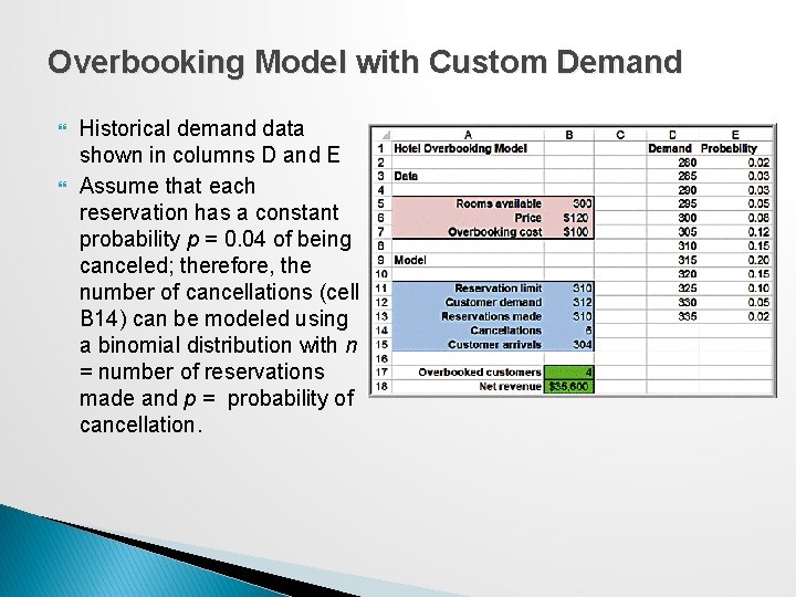
Overbooking Model with Custom Demand Historical demand data shown in columns D and E Assume that each reservation has a constant probability p = 0. 04 of being canceled; therefore, the number of cancellations (cell B 14) can be modeled using a binomial distribution with n = number of reservations made and p = probability of cancellation.

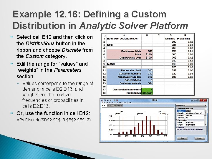
Example 12. 16: Defining a Custom Distribution in Analytic Solver Platform Select cell B 12 and then click on the Distributions button in the ribbon and choose Discrete from the Custom category. Edit the range for “values” and “weights” in the Parameters section ◦ Values correspond to the range of demand in cells D 2: D 13, and weights are the relative frequencies or probabilities in cells E 2: E 13. Or, use the function in cell B 12: =Psi. Discrete($D$2: $D$13, $E$2: $E$13)

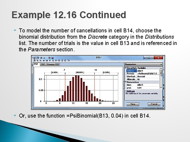
Example 12. 16 Continued To model the number of cancellations in cell B 14, choose the binomial distribution from the Discrete category in the Distributions list. The number of trials is the value in cell B 13 and is referenced in the Parameters section. Or, use the function =Psi. Binomial(B 13, 0. 04) in cell B 14.

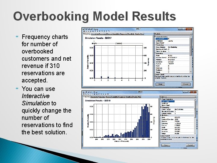
Overbooking Model Results Frequency charts for number of overbooked customers and net revenue if 310 reservations are accepted. You can use Interactive Simulation to quickly change the number of reservations to find the best solution.

Cash Budget Model Cash Budgeting is the process of projecting and summarizing a company’s cash inflows and outflows expected during a planning horizon. � Most cash budgets are based on sales forecasts. �Because of the inherent uncertainty in sales forecasts, Monte Carlo simulation is an appropriate tool for modeling cash budgets.

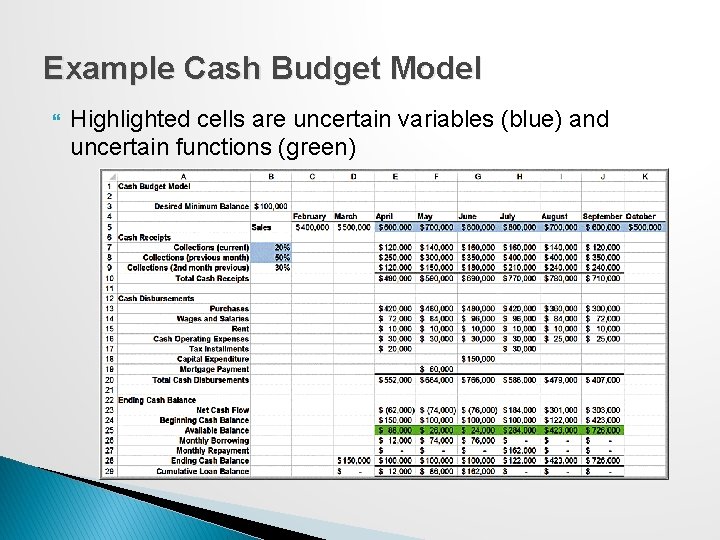
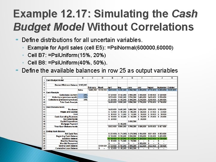
Example Cash Budget Model Highlighted cells are uncertain variables (blue) and uncertain functions (green)

Cash Budget Model Assumptions Sales are normally distributed with a standard deviation of 10% of the mean. Sales in adjacent months are correlated with one another, with a correlation coefficient of 0. 6. On average, 20% of sales are collected in the month of sale, 50%, in the month following the sale, and 30%, in the second month following the sale. ◦ These figures are uncertain, so a uniform distribution is used to model the first two values (15% to 20% and 40% to 50%, respectively), with the assumption that all remaining revenues are collected in the second month following the sale.

Example 12. 17: Simulating the Cash Budget Model Without Correlations Define distributions for all uncertain variables. ◦ Example for April sales (cell E 5): =Psi. Normal(600000, 60000) ◦ Cell B 7: =Psi. Uniform(15%, 20%) ◦ Cell B 8: =Psi. Uniform(40%, 50%). Define the available balances in row 25 as output variables

Example 12. 17 Continued Trend chart

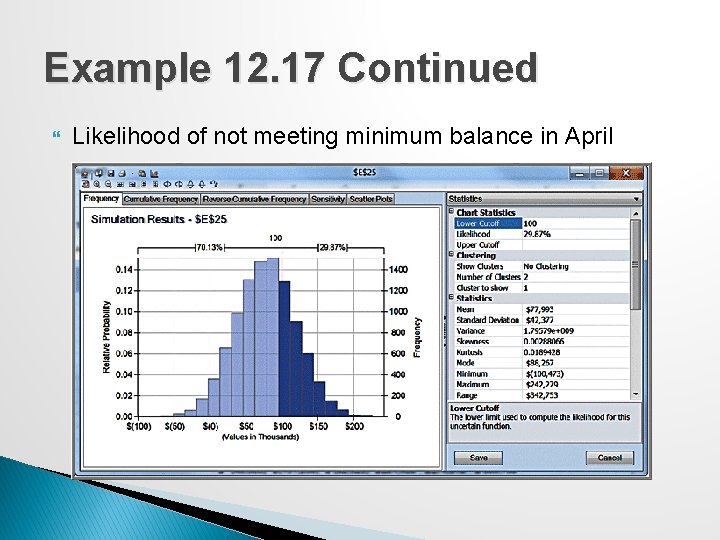
Example 12. 17 Continued Likelihood of not meeting minimum balance in April

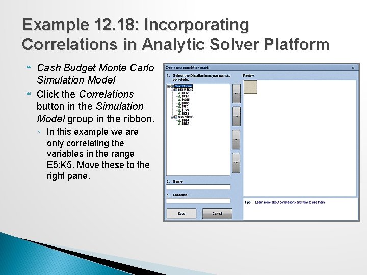
Correlating Uncertain Variables Unless you specify otherwise, Monte Carlo simulation assumes that each of the uncertain variables is independent of all the others. Analytic Solver Platform allows you to specify correlations between uncertain variables.

Example 12. 18: Incorporating Correlations in Analytic Solver Platform Cash Budget Monte Carlo Simulation Model Click the Correlations button in the Simulation Model group in the ribbon. ◦ In this example we are only correlating the variables in the range E 5: K 5. Move these to the right pane.

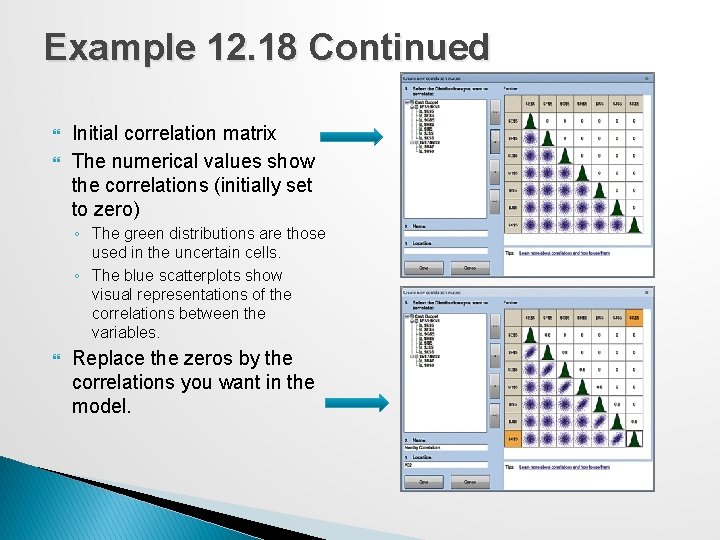
Example 12. 18 Continued Initial correlation matrix The numerical values show the correlations (initially set to zero) ◦ The green distributions are those used in the uncertain cells. ◦ The blue scatterplots show visual representations of the correlations between the variables. Replace the zeros by the correlations you want in the model.

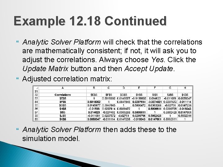
Example 12. 18 Continued Analytic Solver Platform will check that the correlations are mathematically consistent; if not, it will ask you to adjust the correlations. Always choose Yes. Click the Update Matrix button and then Accept Update. Adjusted correlation matrix: Analytic Solver Platform then adds these to the simulation model.