Chapter 12 Monopolistic Competition and Oligopoly Monopolistic Competition

Chapter 12 Monopolistic Competition and Oligopoly

Monopolistic Competition l Characteristics 1. 2. 3. Many firms Free entry and exit Differentiated product © 2005 Pearson Education, Inc. Chapter 12 2

Monopolistic Competition l The amount of monopoly power depends on the degree of differentiation l Examples of this very common market structure include: m Toothpaste m Soap m Cold remedies m Retail © 2005 Pearson Education, Inc. Chapter 12 3

Monopolistic Competition l Two important characteristics m Differentiated but highly substitutable products (cross-price elasticity of demand large) m Free entry and exit (keeps profits down) © 2005 Pearson Education, Inc. Chapter 12 4

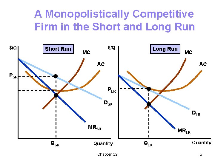
A Monopolistically Competitive Firm in the Short and Long Run $/Q Short Run $/Q MC Long Run MC AC AC PSR PLR DSR DLR MRSR Quantity Chapter 12 MRLR Quantity 5

A Monopolistically Competitive Firm in the Short and Long Run l Short run m Downward sloping demand – differentiated product m Demand is relatively elastic – good substitutes m MR < P m Profits are maximized when MR = MC m This firm is making economic profits © 2005 Pearson Education, Inc. Chapter 12 6

A Monopolistically Competitive Firm in the Short and Long Run l Long run m Profits will attract new firms to the industry (no barriers to entry) m The old firm’s demand will decrease to DLR m Firm’s output and price will fall m Industry output will rise m No economic profit (P = AC) m P > MC some monopoly power © 2005 Pearson Education, Inc. Chapter 12 7

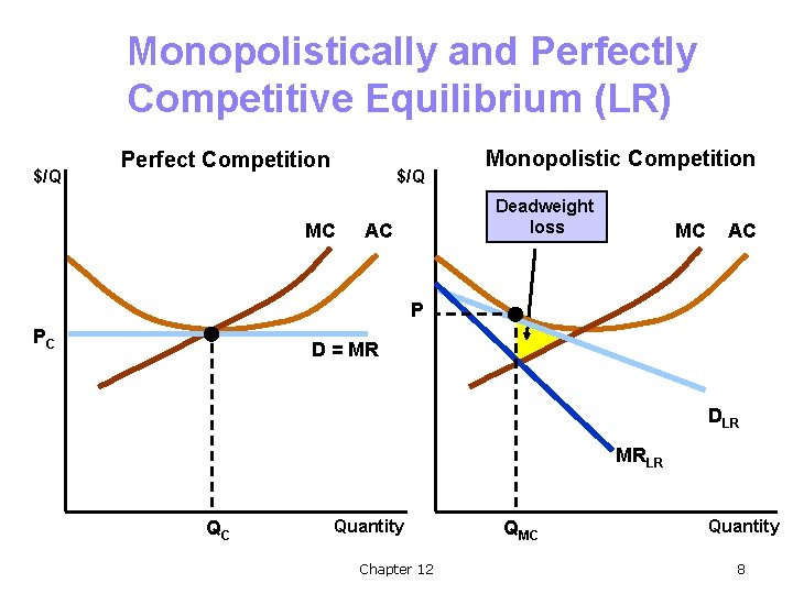
Monopolistically and Perfectly Competitive Equilibrium (LR) $/Q Perfect Competition $/Q MC Monopolistic Competition Deadweight loss AC MC AC P PC D = MR DLR MRLR QC Quantity Chapter 12 QMC Quantity 8

Monopolistic Competition and Economic Efficiency l The monopoly power yields a higher price than perfect competition. If price was lowered to the point where MC = D, consumer surplus would increase by the yellow triangle – deadweight loss. l With no economic profits in the long run, the firm is still not producing at minimum AC and excess capacity exists. © 2005 Pearson Education, Inc. Chapter 12 9

Monopolistic Competition and Economic Efficiency l Firm faces downward sloping demand so zero profit point is to the left of minimum average cost l Excess capacity is inefficient because average cost would be lower with fewer firms © 2005 Pearson Education, Inc. Chapter 12 10

Excess Capacity l The FIRM’s output is inefficiently low: less than minimum ATC l Fewer total firms in the INDUSTRY would increase the FIRM’s demand allow them to take advantage of economies of scale and increase output © 2005 Pearson Education, Inc. Chapter 12 11

Monopolistic Competition l If inefficiency is bad for consumers, should monopolistic competition be regulated? m m Market power is relatively small. Usually there are enough firms to compete with enough substitutability between firms – deadweight loss small. Inefficiency is balanced by benefit of increased product diversity – may easily outweigh deadweight loss. © 2005 Pearson Education, Inc. Chapter 12 12

Oligopoly – Characteristics l Small number of firms l Product differentiation may or may not exist l Barriers to entry m Scale economies m Patents m Technology access ($$) m Name recognition ($$) m Strategic action © 2005 Pearson Education, Inc. Chapter 12 13

Oligopoly l Examples m Automobiles m Steel m Aluminum m Petrochemicals m Electrical © 2005 Pearson Education, Inc. equipment Chapter 12 14

Oligopoly l Management Challenges m Strategic actions to deter entry l Threaten to decrease price against new competitors by keeping excess capacity m Rival behavior l Because only a few firms, each must consider how its actions will affect its rivals and in turn how their rivals will react © 2005 Pearson Education, Inc. Chapter 12 15

Oligopoly – Equilibrium l If one firm decides to cut their price, they must consider what the other firms in the industry will do m Could cut price some, the same amount, or more than firm m Could lead to price war and drastic fall in profits for all l Actions and reactions are dynamic, evolving over time © 2005 Pearson Education, Inc. Chapter 12 16

Oligopoly – Equilibrium l Defining Equilibrium m m Firms are doing the best they can and have no incentive to change their output or price All firms assume competitors are taking rival decisions into account l Nash Equilibrium m Each firm is doing the best it can given what its competitors are doing l We will focus on duopoly m Markets in which two firms compete © 2005 Pearson Education, Inc. Chapter 12 17

Oligopoly l The Cournot Model m Oligopoly model in which firms produce a homogeneous good, each firm treats the output of its competitors as fixed, and all firms decide simultaneously how much to produce m Market price depends on the total output of both firms m Firm will adjust its output based on what it thinks the other firm will produce © 2005 Pearson Education, Inc. Chapter 12 18

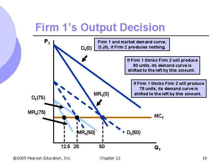
Firm 1’s Output Decision P 1 Firm 1 and market demand curve, D 1(0), if Firm 2 produces nothing. D 1(0) If Firm 1 thinks Firm 2 will produce 50 units, its demand curve is shifted to the left by this amount. MR 1(0) D 1(75) If Firm 1 thinks Firm 2 will produce 75 units, its demand curve is shifted to the left by this amount. MR 1(75) MC 1 MR 1(50) 12. 5 25 © 2005 Pearson Education, Inc. D 1(50) 50 Chapter 12 Q 1 19

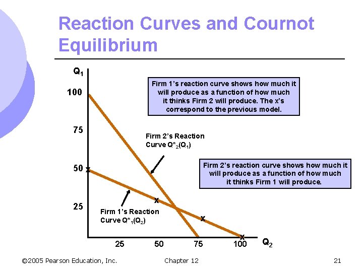
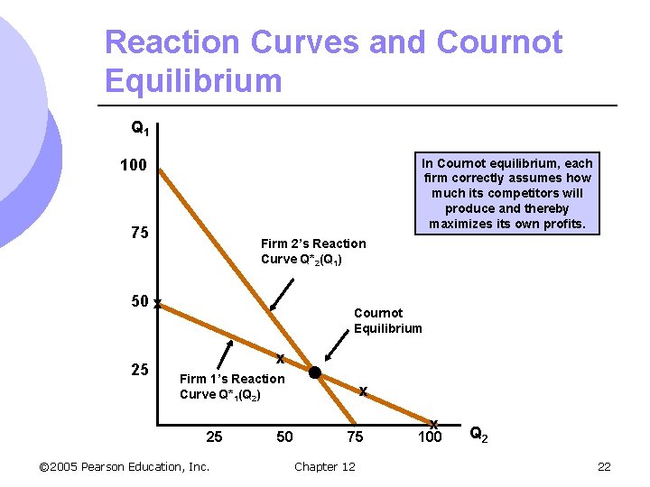
Oligopoly l The Reaction Curve m The relationship between a firm’s profitmaximizing output and the amount it thinks its competitor will produce m A firm’s profit-maximizing output is a decreasing schedule of the expected output of Firm 2 m Different MC = different reaction functions © 2005 Pearson Education, Inc. Chapter 12 20

Reaction Curves and Cournot Equilibrium Q 1 Firm 1’s reaction curve shows how much it will produce as a function of how much it thinks Firm 2 will produce. The x’s correspond to the previous model. 100 75 Firm 2’s Reaction Curve Q*2(Q 1) Firm 2’s reaction curve shows how much it will produce as a function of how much it thinks Firm 1 will produce. 50 x 25 x Firm 1’s Reaction Curve Q*1(Q 2) 25 © 2005 Pearson Education, Inc. 50 x 75 Chapter 12 x 100 Q 2 21

Reaction Curves and Cournot Equilibrium Q 1 100 In Cournot equilibrium, each firm correctly assumes how much its competitors will produce and thereby maximizes its own profits. 75 Firm 2’s Reaction Curve Q*2(Q 1) 50 x 25 Cournot Equilibrium x Firm 1’s Reaction Curve Q*1(Q 2) 25 © 2005 Pearson Education, Inc. 50 x 75 Chapter 12 x 100 Q 2 22

Cournot Equilibrium l Each firm’s reaction curve tells it how much to produce given the output of its competitor l Equilibrium in the Cournot model, in which each firm correctly assumes how much its competitor will produce and sets its own production level accordingly © 2005 Pearson Education, Inc. Chapter 12 23

Oligopoly l Cournot equilibrium is an example of a Nash equilibrium (Cournot-Nash Equilibrium) l The Cournot equilibrium says nothing about the dynamics of the adjustment process m Since both firms adjust their output, neither output would be fixed © 2005 Pearson Education, Inc. Chapter 12 24

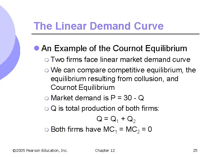
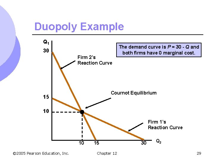
The Linear Demand Curve l An Example of the Cournot Equilibrium m Two firms face linear market demand curve m We can compare competitive equilibrium, the equilibrium resulting from collusion, and Cournot Equilibrium m Market demand is P = 30 - Q m Q is total production of both firms: Q = Q 1 + Q 2 m Both firms have MC 1 = MC 2 = 0 © 2005 Pearson Education, Inc. Chapter 12 25

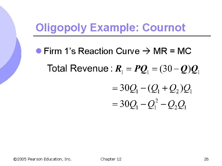
Oligopoly Example: Cournot l Firm 1’s Reaction Curve MR = MC © 2005 Pearson Education, Inc. Chapter 12 26

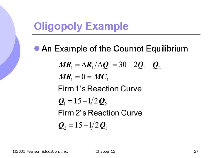
Oligopoly Example l An Example of the Cournot Equilibrium © 2005 Pearson Education, Inc. Chapter 12 27

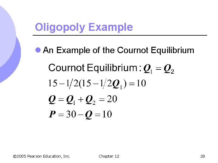
Oligopoly Example l An Example of the Cournot Equilibrium © 2005 Pearson Education, Inc. Chapter 12 28

Duopoly Example Q 1 30 Firm 2’s Reaction Curve The demand curve is P = 30 - Q and both firms have 0 marginal cost. Cournot Equilibrium 15 10 Firm 1’s Reaction Curve 10 © 2005 Pearson Education, Inc. 15 Chapter 12 30 Q 2 29

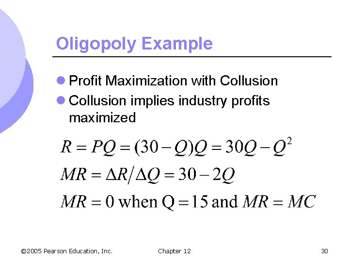
Oligopoly Example l Profit Maximization with Collusion l Collusion implies industry profits maximized © 2005 Pearson Education, Inc. Chapter 12 30

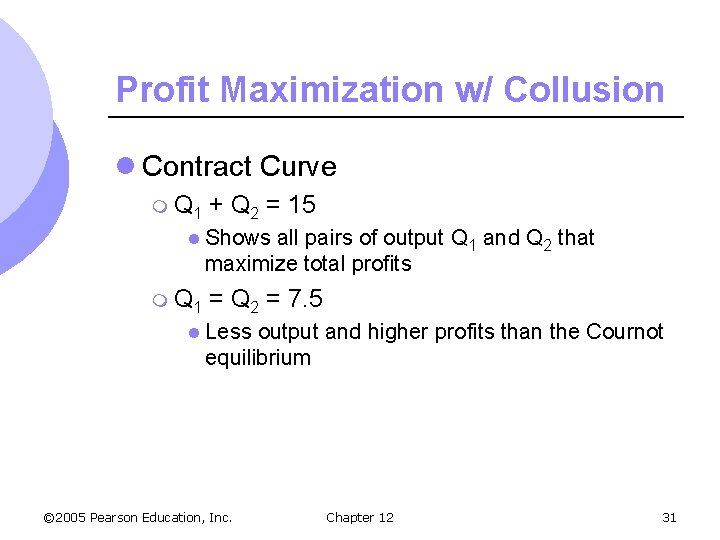
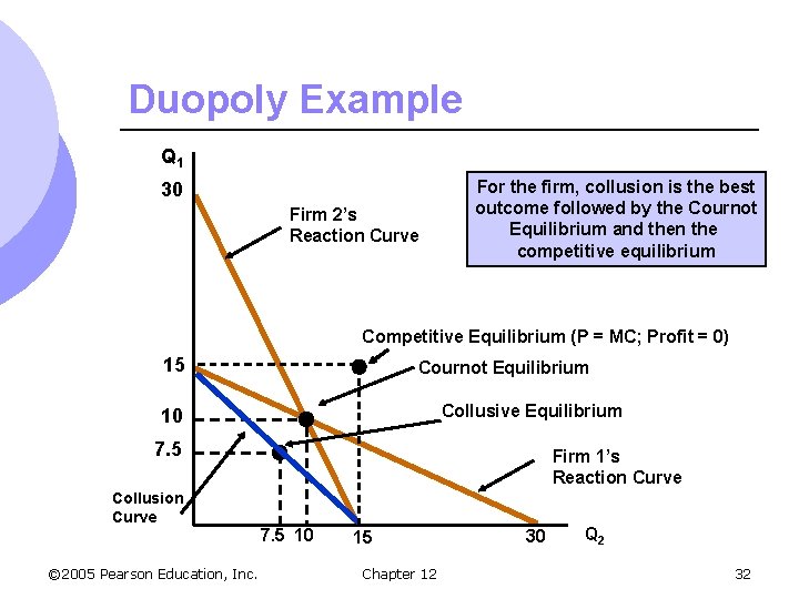
Profit Maximization w/ Collusion l Contract Curve m Q 1 + Q 2 = 15 l Shows all pairs of output Q 1 and Q 2 that maximize total profits m Q 1 = Q 2 = 7. 5 l Less output and higher profits than the Cournot equilibrium © 2005 Pearson Education, Inc. Chapter 12 31

Duopoly Example Q 1 30 Firm 2’s Reaction Curve For the firm, collusion is the best outcome followed by the Cournot Equilibrium and then the competitive equilibrium Competitive Equilibrium (P = MC; Profit = 0) 15 Cournot Equilibrium Collusive Equilibrium 10 7. 5 Collusion Curve © 2005 Pearson Education, Inc. Firm 1’s Reaction Curve 7. 5 10 15 Chapter 12 30 Q 2 32

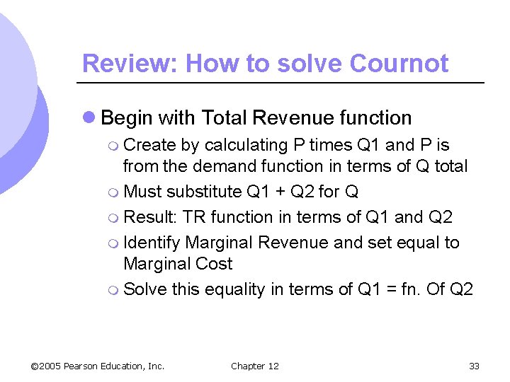
Review: How to solve Cournot l Begin with Total Revenue function m Create by calculating P times Q 1 and P is from the demand function in terms of Q total m Must substitute Q 1 + Q 2 for Q m Result: TR function in terms of Q 1 and Q 2 m Identify Marginal Revenue and set equal to Marginal Cost m Solve this equality in terms of Q 1 = fn. Of Q 2 © 2005 Pearson Education, Inc. Chapter 12 33

First Mover Advantage – The Stackelberg Model l Oligopoly model in which one firm sets its output before other firms do l Assumptions m One firm can set output first m MC = 0 m Market demand is P = 30 - Q where Q is total output m Firm 1 sets output first and Firm 2 then makes an output decision seeing Firm 1’s output © 2005 Pearson Education, Inc. Chapter 12 34

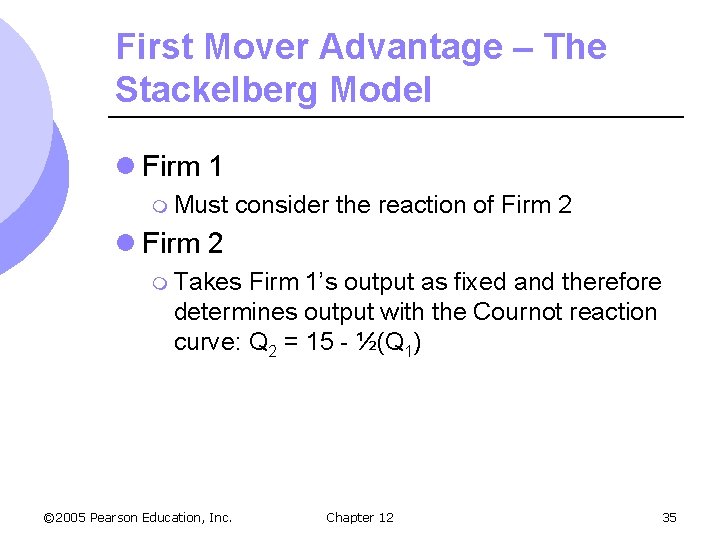
First Mover Advantage – The Stackelberg Model l Firm 1 m Must consider the reaction of Firm 2 l Firm 2 m Takes Firm 1’s output as fixed and therefore determines output with the Cournot reaction curve: Q 2 = 15 - ½(Q 1) © 2005 Pearson Education, Inc. Chapter 12 35

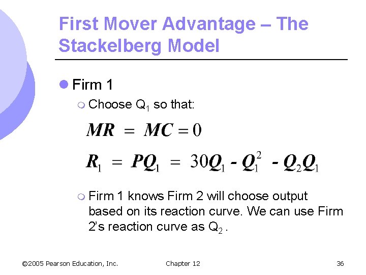
First Mover Advantage – The Stackelberg Model l Firm 1 m Choose Q 1 so that: m Firm 1 knows Firm 2 will choose output based on its reaction curve. We can use Firm 2’s reaction curve as Q 2. © 2005 Pearson Education, Inc. Chapter 12 36

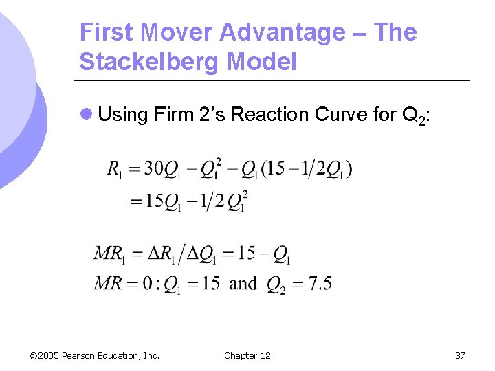
First Mover Advantage – The Stackelberg Model l Using Firm 2’s Reaction Curve for Q 2: © 2005 Pearson Education, Inc. Chapter 12 37

First Mover Advantage – The Stackelberg Model l Conclusion m Going first gives Firm 1 the advantage m Firm 1’s output is twice as large as Firm 2’s m Firm 1’s profit is twice as large as Firm 2’s l Going first allows Firm 1 to produce a large quantity. Firm 2 must take that into account and produce less unless it wants to reduce profits for everyone. © 2005 Pearson Education, Inc. Chapter 12 38

Price Competition l Competition in an oligopolistic industry may occur with price instead of output l The Bertrand Model is used m Oligopoly model in which firms produce a homogeneous good, each firm treats the price of its competitors as fixed, and all firms decide simultaneously what price to charge © 2005 Pearson Education, Inc. Chapter 12 39

Price Competition – Bertrand Model l Assumptions m Homogenous good m Market demand is P = 30 - Q where Q = Q 1 + Q 2 m MC 1 = MC 2 = $3 l Can show the Cournot equilibrium if Q 1 = Q 2 = 9 and market price is $12, giving each firm a profit of $81. © 2005 Pearson Education, Inc. Chapter 12 40

Price Competition – Bertrand Model l Assume here that the firms compete with price, not quantity l Since good is homogeneous, consumers will buy from lowest price seller m If firms charge different prices, consumers buy from lowest priced firm only m If firms charge same price, consumers are indifferent who they buy from and each firm will supply half the market © 2005 Pearson Education, Inc. Chapter 12 41

Price Competition – Bertrand Model l Nash equilibrium is competitive equilibrium output since have incentive to cut prices l Both firms set price equal to MC m. P = MC; P 1 = P 2 = $3 m Q = 27; Q 1 & Q 2 = 13. 5 l Both firms earn zero profit © 2005 Pearson Education, Inc. Chapter 12 42

Price Competition – Bertrand Model l Why not charge a different price? m If charge more, sell nothing m If charge less, lose money on each unit sold l The Bertrand model demonstrates the importance of the strategic variable m Price © 2005 Pearson Education, Inc. versus output Chapter 12 43

Bertrand Model – Criticisms l When firms produce a homogenous good, it is more natural to compete by setting quantities rather than prices l Even if the firms do choose the same price, what share of total sales will go to each one? m Probably © 2005 Pearson Education, Inc. not exactly half Chapter 12 44

Competition Versus Collusion: The Prisoners’ Dilemma l Nash equilibrium is a noncooperative equilibrium: each firm makes decision that gives greatest profit, given actions of competitors l Although collusion is illegal, why don’t firms cooperate without explicitly colluding? m Why not set profit maximizing collusion price and hope others follow? © 2005 Pearson Education, Inc. Chapter 12 45

Competition Versus Collusion: The Prisoners’ Dilemma l Competitor is not likely to follow l Competitor can do better by choosing a lower price, even if they know you will set the collusive level price l We can use a payoff matrix to better understand the firms’ choices © 2005 Pearson Education, Inc. Chapter 12 46

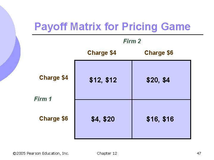
Payoff Matrix for Pricing Game Firm 2 Charge $4 Charge $6 $12, $12 $20, $4 $4, $20 $16, $16 Firm 1 Charge $6 © 2005 Pearson Education, Inc. Chapter 12 47

Competition Versus Collusion: The Prisoners’ Dilemma l We can now answer the question of why firm does not choose cooperative price l Cooperating means both firms charging $6 instead of $4 and earning $16 instead of $12 l Each firm always makes more money by charging $4, no matter what its competitor does l Unless enforceable agreement to charge $6, will be better off charging $4 © 2005 Pearson Education, Inc. Chapter 12 48

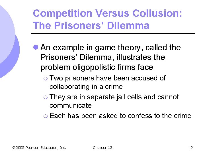
Competition Versus Collusion: The Prisoners’ Dilemma l An example in game theory, called the Prisoners’ Dilemma, illustrates the problem oligopolistic firms face m Two prisoners have been accused of collaborating in a crime m They are in separate jail cells and cannot communicate m Each has been asked to confess to the crime © 2005 Pearson Education, Inc. Chapter 12 49

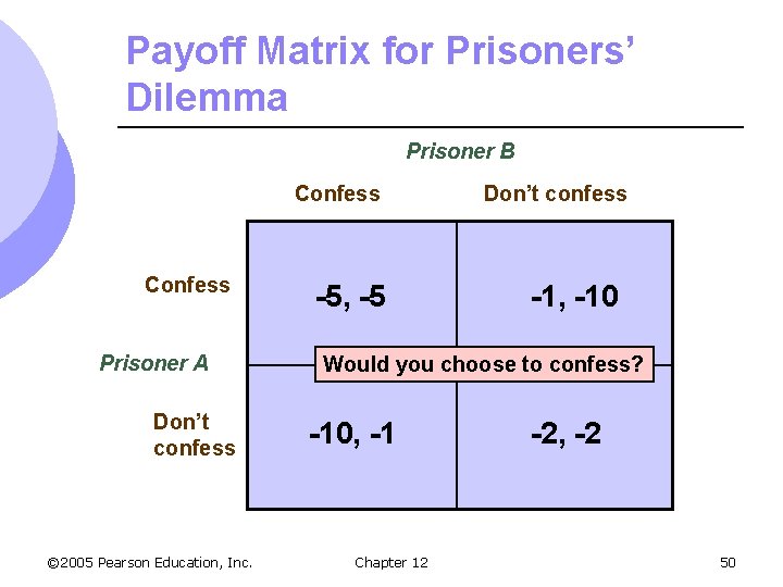
Payoff Matrix for Prisoners’ Dilemma Prisoner B Confess Prisoner A Don’t confess © 2005 Pearson Education, Inc. -5, -5 Don’t confess -1, -10 Would you choose to confess? -10, -1 Chapter 12 -2, -2 50

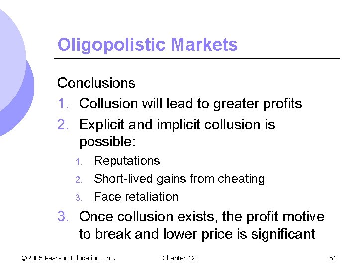
Oligopolistic Markets Conclusions 1. Collusion will lead to greater profits 2. Explicit and implicit collusion is possible: 1. 2. 3. Reputations Short-lived gains from cheating Face retaliation 3. Once collusion exists, the profit motive to break and lower price is significant © 2005 Pearson Education, Inc. Chapter 12 51

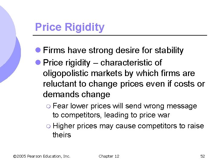
Price Rigidity l Firms have strong desire for stability l Price rigidity – characteristic of oligopolistic markets by which firms are reluctant to change prices even if costs or demands change m Fear lower prices will send wrong message to competitors, leading to price war m Higher prices may cause competitors to raise theirs © 2005 Pearson Education, Inc. Chapter 12 52

Price Rigidity l Basis of kinked demand curve model of oligopoly m Each firm faces a demand curve kinked at the current prevailing price, P* m Above P*, demand is very elastic l If P > P*, other firms will not follow m Below l If P*, demand is very inelastic P < P*, other firms will follow suit © 2005 Pearson Education, Inc. Chapter 12 53

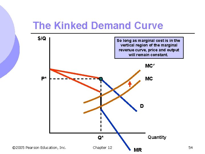
The Kinked Demand Curve $/Q So long as marginal cost is in the vertical region of the marginal revenue curve, price and output will remain constant. MC’ P* MC D Quantity Q* © 2005 Pearson Education, Inc. Chapter 12 MR 54

Price Rigidity l With a kinked demand curve, marginal revenue curve is discontinuous l Firm’s costs can change without resulting in a change in price l Kinked demand curve does not really explain oligopolistic pricing m Description of price rigidity rather than an explanation of it m How was price chosen to begin with? © 2005 Pearson Education, Inc. Chapter 12 55

Price Signaling and Price Leadership l Price Signaling m Implicit collusion in which a firm announces a price increase in the hope that other firms will follow suit l Price Leadership m Pattern of pricing in which one firm regularly announces price changes that other firms then match © 2005 Pearson Education, Inc. Chapter 12 56

Cartels l Producers in a cartel explicitly agree to cooperate in setting prices and output l Typically only a subset of producers are part of the cartel and others benefit from the choices of the cartel l If demand is sufficiently inelastic and cartel is enforceable, prices may be well above competitive levels l Most fail to maintain high prices © 2005 Pearson Education, Inc. Chapter 12 57

Cartels l Examples of successful cartels m m m OPEC International Bauxite Association Mercurio Europeo l Examples of unsuccessful cartels m m m © 2005 Pearson Education, Inc. Chapter 12 Copper Tin Coffee Tea Cocoa 58

Cartels – Conditions for Success 1. Stable cartel organization must be formed – price and quantity settled on and adhered to m m Members have different costs, assessments of demand objectives Tempting to cheat by lowering price to capture larger market share © 2005 Pearson Education, Inc. Chapter 12 59

Cartels – Conditions for Success 2. Potential for monopoly power m m m Even if cartel can succeed, there might be little room to raise prices if it faces highly elastic demand If potential gains from cooperation are large, cartel members will have more incentive to make the cartel work Low potential = low incentive to work out organizational problems © 2005 Pearson Education, Inc. Chapter 12 60

Cartels l To be successful: m Total demand must be fairly inelastic m Either the cartel must control nearly all of the world’s supply or the supply of noncartel producers must also be inelastic © 2005 Pearson Education, Inc. Chapter 12 61

The Cartelization of Intercollegiate Athletics 1. Large number of firms (colleges) 2. Large number of consumers (fans) 3. Very high profits © 2005 Pearson Education, Inc. Chapter 12 62

The Cartelization of Intercollegiate Athletics l NCAA is the cartel m Restricts competition m Reduces bargaining power by athletes – enforces rules regarding eligibility and terms of compensation m Reduces competition by universities – limits number of games played each season, number of teams per division, etc. m Limits price competition – sole negotiator for all football television contracts © 2005 Pearson Education, Inc. Chapter 12 63

The Cartelization of Intercollegiate Athletics l Although members have occasionally broken rules and regulations, has been a successful cartel l In 1984, Supreme Court ruled that the NCAA’s monopolization of football TV contracts was illegal m Competition led to drop in contract fees m More college football on TV, but lower revenues to schools © 2005 Pearson Education, Inc. Chapter 12 64