Chapter 12 Introduction to Binomial Trees Chapter 12
Chapter 12 Introduction to Binomial Trees Chapter 12 1
Intro. To Binomial Trees • Binomial Tree – A diagram representing different possible paths that might be followed by the stock price over the life of the option. – Five things will always be given…. 1. Stock price 2. Upward movement and Downward movement 3. Risk-free rate 4. strike price 5. and maturity Chapter 12 2
Intro. To Binomial Trees • No Arbitrage Assumption • Riskless portfolio • A portfolio of stocks and option that has no uncertainty about the value of the portfolio at maturity is called riskless portfolio. The return on the riskless portfolio is called risk-free return. 1 step binomial $ change 1 time 2 step binomial $ change 2 times Chapter 12 3

Class Exercise 12 Chapter 12 4
A Simple Binomial Model Steps to price the option • A stock price is currently $20. It is known that at the end of one month it will be either $22 or $18. The risk-free rate is 12% per annum with continuous compounding. What is the value of three-month European call option with strike price $21? Chapter 12 5
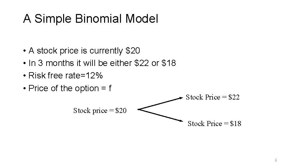
A Simple Binomial Model • A stock price is currently $20 • In 3 months it will be either $22 or $18 • Risk free rate=12% • Price of the option = f Stock Price = $22 Stock price = $20 Stock Price = $18 6
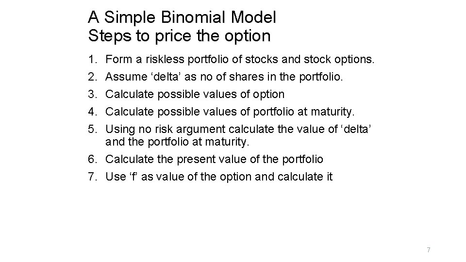
A Simple Binomial Model Steps to price the option 1. 2. 3. 4. 5. Form a riskless portfolio of stocks and stock options. Assume ‘delta’ as no of shares in the portfolio. Calculate possible values of option Calculate possible values of portfolio at maturity. Using no risk argument calculate the value of ‘delta’ and the portfolio at maturity. 6. Calculate the present value of the portfolio 7. Use ‘f’ as value of the option and calculate it 7
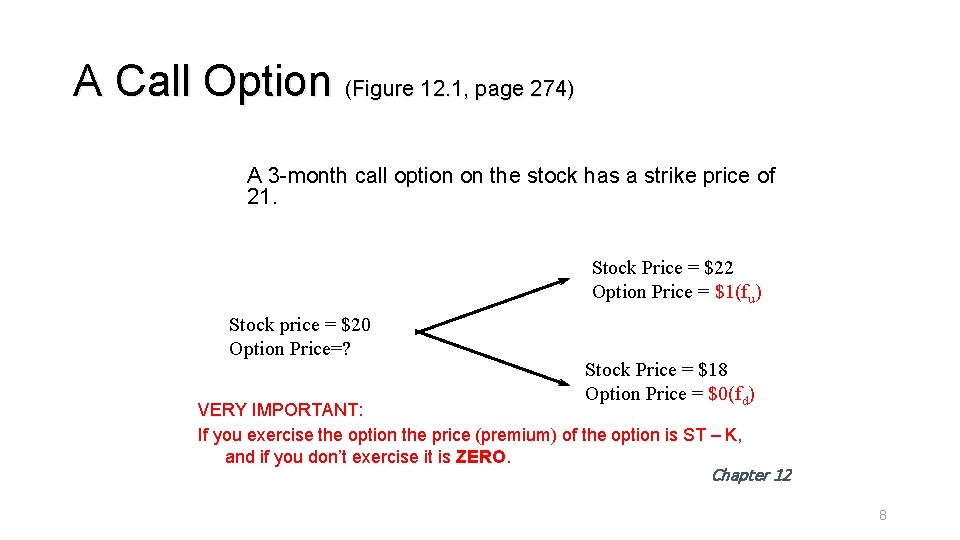
A Call Option (Figure 12. 1, page 274) A 3 -month call option on the stock has a strike price of 21. Stock Price = $22 Option Price = $1(fu) Stock price = $20 Option Price=? Stock Price = $18 Option Price = $0(fd) VERY IMPORTANT: If you exercise the option the price (premium) of the option is ST – K, and if you don’t exercise it is ZERO. Chapter 12 8
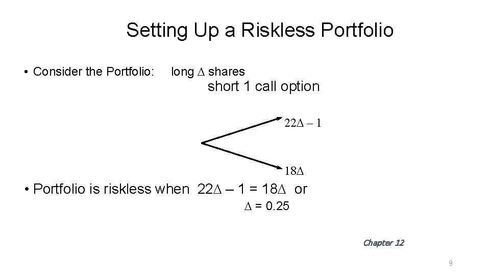
Setting Up a Riskless Portfolio • Consider the Portfolio: long D shares short 1 call option 22 D – 1 18 D • Portfolio is riskless when 22 D – 1 = 18 D or D = 0. 25 Chapter 12 9
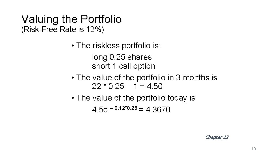
Valuing the Portfolio (Risk-Free Rate is 12%) • The riskless portfolio is: long 0. 25 shares short 1 call option • The value of the portfolio in 3 months is 22 * 0. 25 – 1 = 4. 50 • The value of the portfolio today is 4. 5 e – 0. 12*0. 25 = 4. 3670 Chapter 12 10
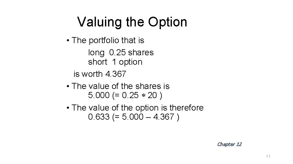
Valuing the Option • The portfolio that is long 0. 25 shares short 1 option is worth 4. 367 • The value of the shares is 5. 000 (= 0. 25 * 20 ) • The value of the option is therefore 0. 633 (= 5. 000 – 4. 367 ) Chapter 12 11
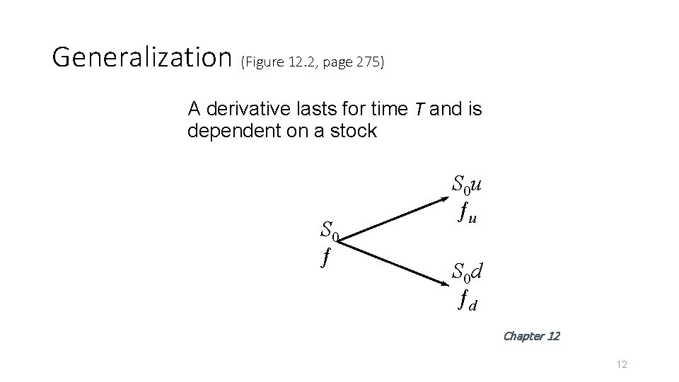
Generalization (Figure 12. 2, page 275) A derivative lasts for time T and is dependent on a stock S 0 ƒ S 0 u ƒu S 0 d ƒd Chapter 12 12
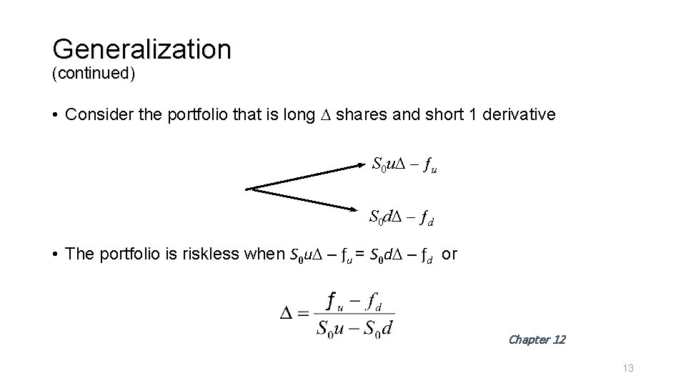
Generalization (continued) • Consider the portfolio that is long D shares and short 1 derivative S 0 u. D – ƒu S 0 d. D – ƒd • The portfolio is riskless when S 0 u. D – ƒu = S 0 d. D – ƒd or Chapter 12 13
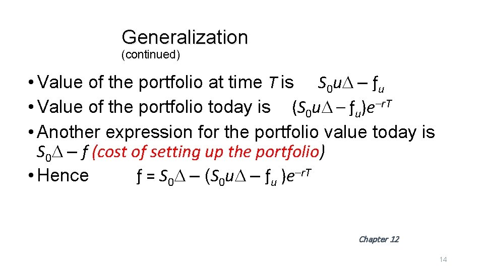
Generalization (continued) • Value of the portfolio at time T is S 0 u. D – ƒu • Value of the portfolio today is (S 0 u. D – ƒu)e–r. T • Another expression for the portfolio value today is S 0 D – f (cost of setting up the portfolio) • Hence ƒ = S 0 D – (S 0 u. D – ƒu )e–r. T Chapter 12 14
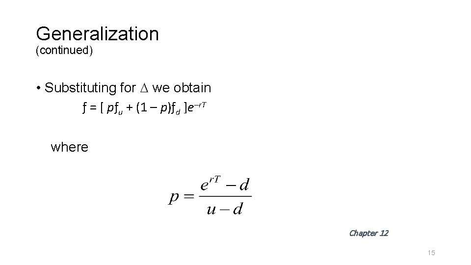
Generalization (continued) • Substituting for D we obtain ƒ = [ pƒu + (1 – p)ƒd ]e–r. T where Chapter 12 15
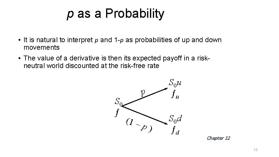
p as a Probability • It is natural to interpret p and 1 -p as probabilities of up and down movements • The value of a derivative is then its expected payoff in a riskneutral world discounted at the risk-free rate S 0 ƒ (1 – p S 0 u ƒu p) S 0 d ƒd Chapter 12 16
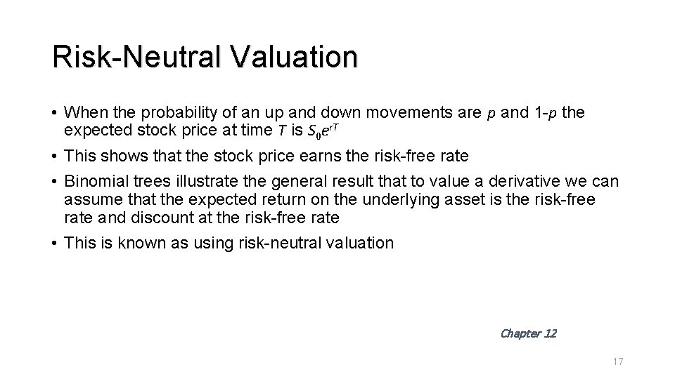
Risk-Neutral Valuation • When the probability of an up and down movements are p and 1 -p the expected stock price at time T is S 0 er. T • This shows that the stock price earns the risk-free rate • Binomial trees illustrate the general result that to value a derivative we can assume that the expected return on the underlying asset is the risk-free rate and discount at the risk-free rate • This is known as using risk-neutral valuation Chapter 12 17
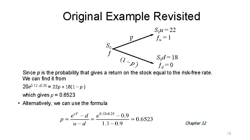
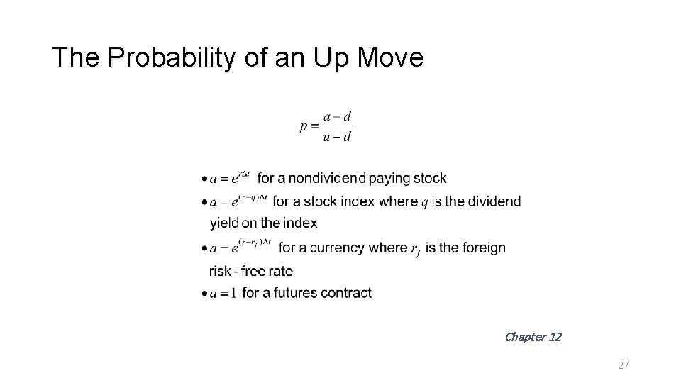
Original Example Revisited p S 0 ƒ (1 – p) S 0 u = 22 ƒu = 1 S 0 d = 18 ƒd = 0 Since p is the probability that gives a return on the stock equal to the risk-free rate. We can find it from 20 e 0. 12 ´ 0. 25 = 22 p + 18(1 – p ) which gives p = 0. 6523 • Alternatively, we can use the formula Chapter 12 18
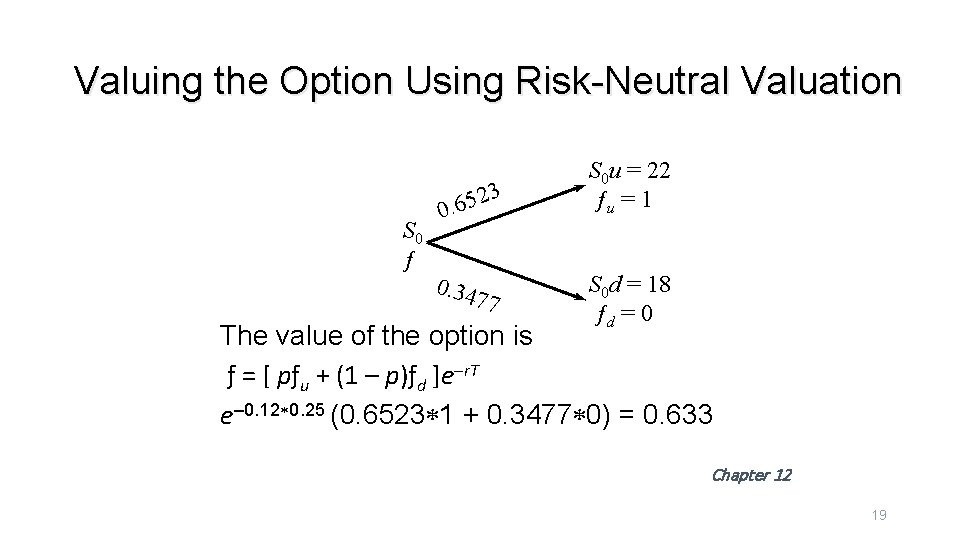
Valuing the Option Using Risk-Neutral Valuation S 0 ƒ 23 5 6. 0 0. 34 77 S 0 u = 22 ƒu = 1 S 0 d = 18 ƒd = 0 The value of the option is ƒ = [ pƒu + (1 – p)ƒd ]e–r. T e– 0. 12*0. 25 (0. 6523*1 + 0. 3477*0) = 0. 633 Chapter 12 19
Irrelevance of Stock’s Expected Return • • When we are valuing an option in terms of the price of the underlying asset, the probability of up and down movements in the real world are irrelevant This is an example of a more general result stating that the expected return on the underlying asset in the real world is irrelevant Chapter 12 20
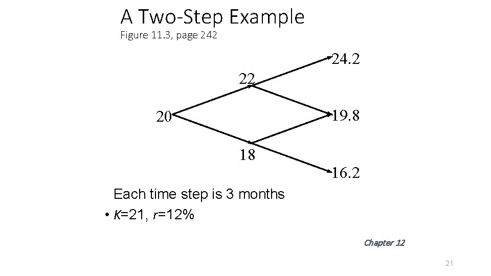
A Two-Step Example Figure 11. 3, page 242 24. 2 22 19. 8 20 18 16. 2 Each time step is 3 months • K=21, r=12% Chapter 12 21
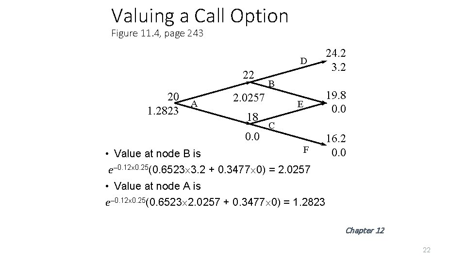
Valuing a Call Option Figure 11. 4, page 243 D 22 20 1. 2823 A B 2. 0257 18 0. 0 E 24. 2 3. 2 19. 8 0. 0 C F • Value at node B is e– 0. 12´ 0. 25(0. 6523´ 3. 2 + 0. 3477´ 0) = 2. 0257 16. 2 0. 0 • Value at node A is e– 0. 12´ 0. 25(0. 6523´ 2. 0257 + 0. 3477´ 0) = 1. 2823 Chapter 12 22
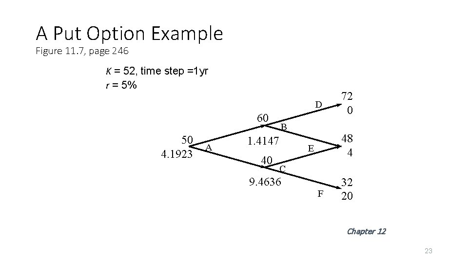
A Put Option Example Figure 11. 7, page 246 K = 52, time step =1 yr r = 5% D 60 50 4. 1923 A B 1. 4147 40 72 0 48 4 E C 9. 4636 F 32 20 Chapter 12 23
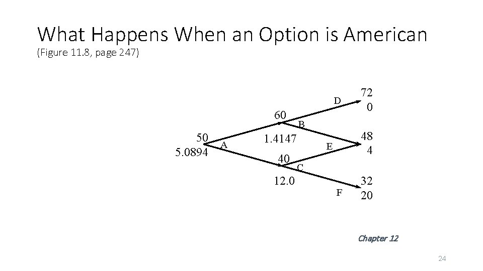
What Happens When an Option is American (Figure 11. 8, page 247) D 60 50 5. 0894 A B 1. 4147 40 12. 0 72 0 48 4 E C F 32 20 Chapter 12 24
Delta • Delta (D) is the ratio of the change in the price of a stock option to the change in the price of the underlying stock • The value of D varies from node to node Chapter 12 25

Choosing u and d One way of matching the volatility is to set where s is the volatility and Dt is the length of the time step. This is the approach used by Cox, Ross, and Rubinstein Chapter 12 26
The Probability of an Up Move Chapter 12 27
- Slides: 27