Chapter 12 Independent Demand Inventory Management Operations Management

Chapter 12 – Independent Demand Inventory Management Operations Management by R. Dan Reid & Nada R. Sanders 4 th Edition © Wiley 2010 Power. Point Presentation by R. B. Clough – UNH M. E. Henrie - UAA © Wiley 2010

Wall Street Speaks (compiled by Teradata, a division of NCR) n n “Shares of Intel Corp. fell to an 11 -month low on Wednesday, leading a decline in semiconductor-industry stocks a day after the world’s largest chipmaker warned that its inventories had risen sharply”, this despite 96% growth in quarterly profit. –Reuters, July 14, 2004 “Cisco Systems Inc. on Tuesday reported that quarterly profit surges 41%, but its shares fell sharply in after-hours trade on a rise in inventories. ” - Reuters, August 10, 2004 © Wiley 2010

Wall Street Speaks (compiled by Teradata, a division of NCR) n n n “The day Nike announced the breakdown in its chain, the company’s stock dropped 20%, an amount so staggering that it makes the $100 million loss (in sales) seem like pocket change. ” – Computer World, November 10, 2003 “General Motors was down 3. 1%, or $1. 37, at $42. 75, after analysts with Goldman Sachs and Lehman Brothers downgraded their ratings of the stock, amid worries of inventory buildup. ” –AP, July 30, 2004 “Blind execution [of a production plan] in the face of variation can tie up hundreds of millions in working capital and prevent you from supporting customer demand. ” -Teradata © Wiley 2010

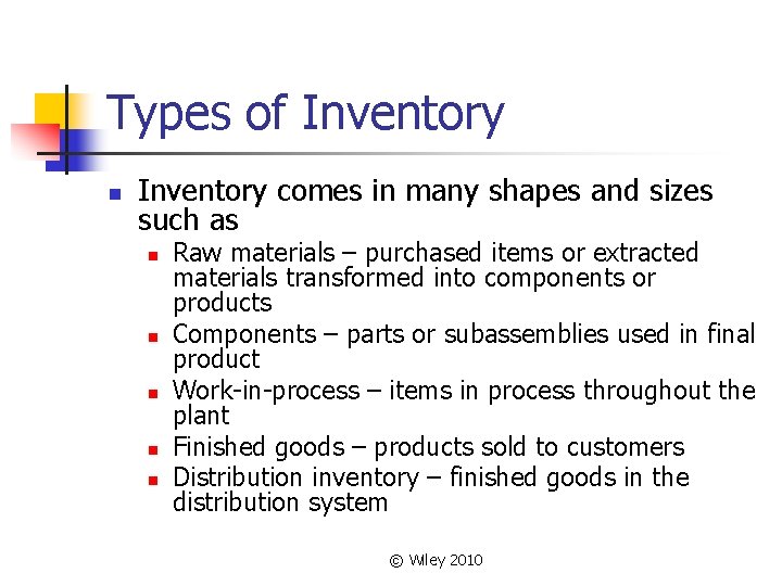
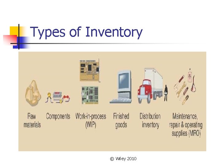
Types of Inventory n Inventory comes in many shapes and sizes such as n n n Raw materials – purchased items or extracted materials transformed into components or products Components – parts or subassemblies used in final product Work-in-process – items in process throughout the plant Finished goods – products sold to customers Distribution inventory – finished goods in the distribution system © Wiley 2010

Types of Inventory © Wiley 2010

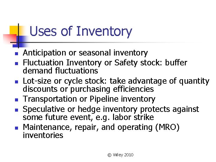
Uses of Inventory n n n Anticipation or seasonal inventory Fluctuation Inventory or Safety stock: buffer demand fluctuations Lot-size or cycle stock: take advantage of quantity discounts or purchasing efficiencies Transportation or Pipeline inventory Speculative or hedge inventory protects against some future event, e. g. labor strike Maintenance, repair, and operating (MRO) inventories © Wiley 2010

Principal Quantitative Models in Ch. 12 Inventory Turnover & Days or Weeks of Supply n P-Models: Periodic Review Models n Q-Models: Continuous Review Models n ABC Classification n © Wiley 2010

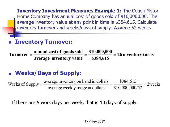
Inventory Investment Measures Example 1: The Coach Motor Home Company has annual cost of goods sold of $10, 000. The average inventory value at any point in time is $384, 615. Calculate inventory turnover and weeks/days of supply. Assume 52 weeks. n Inventory Turnover: n Weeks/Days of Supply: If there are 5 work days per week, that is 10 days of supply. © Wiley 2010

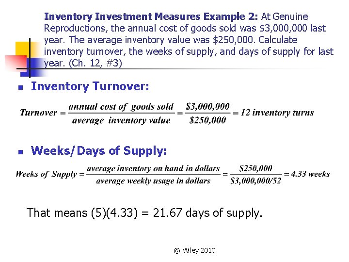
Inventory Investment Measures Example 2: At Genuine Reproductions, the annual cost of goods sold was $3, 000 last year. The average inventory value was $250, 000. Calculate inventory turnover, the weeks of supply, and days of supply for last year. (Ch. 12, #3) n Inventory Turnover: n Weeks/Days of Supply: That means (5)(4. 33) = 21. 67 days of supply. © Wiley 2010

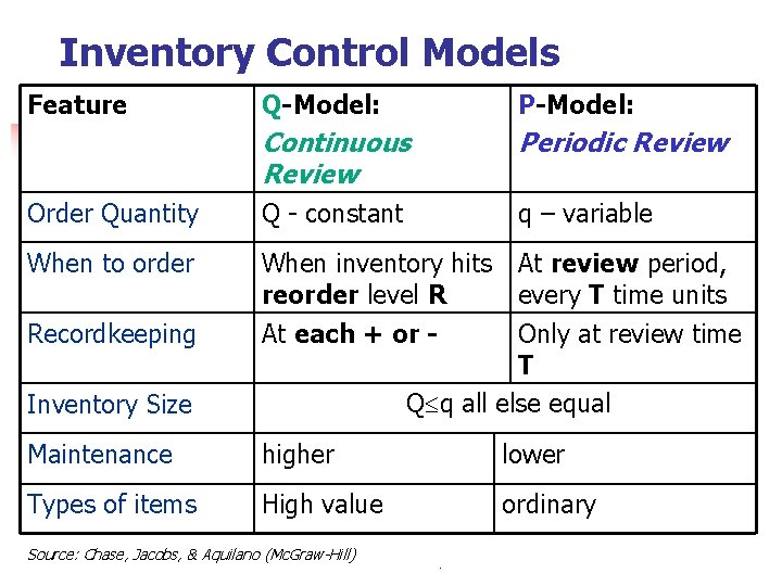
Inventory Control Models Feature Q-Model: P-Model: Continuous Review Periodic Review Order Quantity Q - constant q – variable When to order When inventory hits reorder level R At each + or - Recordkeeping At review period, every T time units Only at review time T Q q all else equal Inventory Size Maintenance higher lower Types of items High value ordinary Source: Chase, Jacobs, & Aquilano (Mc. Graw-Hill) © Wiley 2010

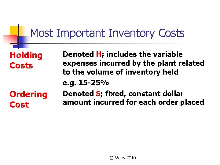
Most Important Inventory Costs Holding Costs Denoted H; includes the variable expenses incurred by the plant related to the volume of inventory held e. g. 15 -25% Ordering Cost Denoted S; fixed, constant dollar amount incurred for each order placed © Wiley 2010

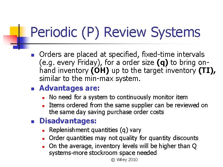
Periodic (P) Review Systems n n Orders are placed at specified, fixed-time intervals (e. g. every Friday), for a order size (q) to bring onhand inventory (OH) up to the target inventory (TI), similar to the min-max system. Advantages are: n n n No need for a system to continuously monitor item Items ordered from the same supplier can be reviewed on the same day saving purchase order costs Disadvantages: n n n Replenishment quantities (q) vary Order quantities may not quality for quantity discounts On the average, inventory levels will be higher than Q systems-more stockroom space needed © Wiley 2010

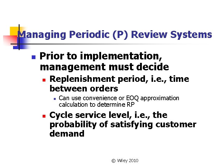
Managing Periodic (P) Review Systems n Prior to implementation, management must decide n Replenishment period, i. e. , time between orders n n Can use convenience or EOQ approximation calculation to determine RP Cycle service level, i. e. , the probability of satisfying customer demand © Wiley 2010

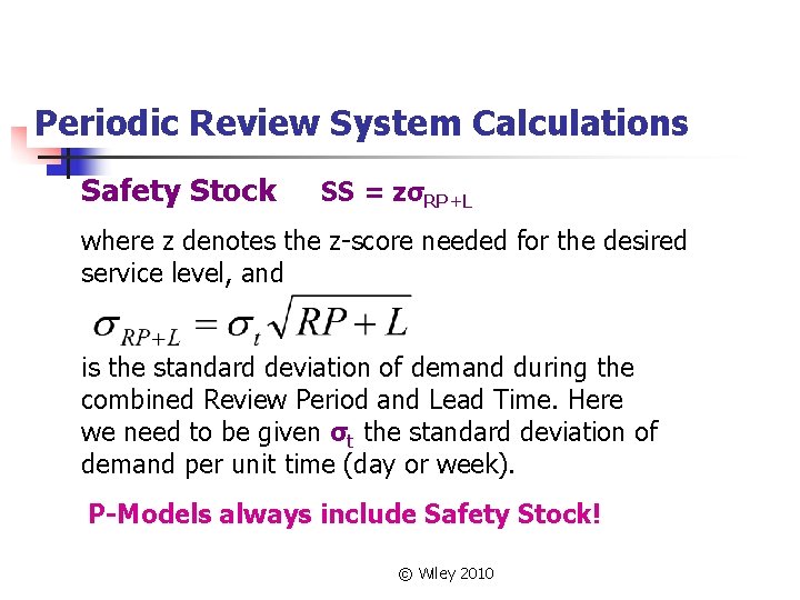
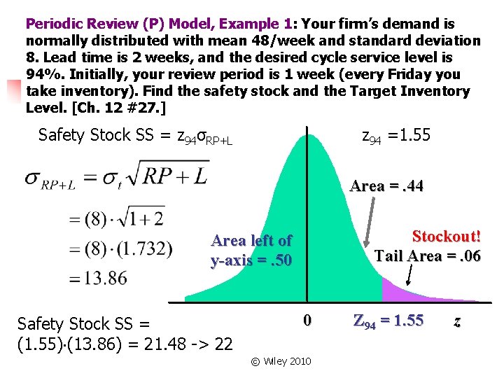
Periodic Review System Calculations Safety Stock SS = zσRP+L where z denotes the z-score needed for the desired service level, and is the standard deviation of demand during the combined Review Period and Lead Time. Here we need to be given σt the standard deviation of demand per unit time (day or week). P-Models always include Safety Stock! © Wiley 2010

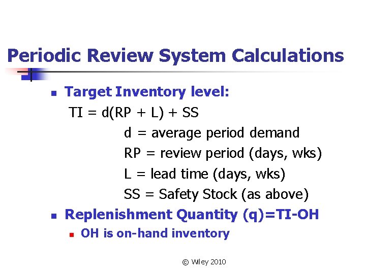
Periodic Review System Calculations n n Target Inventory level: TI = d(RP + L) + SS d = average period demand RP = review period (days, wks) L = lead time (days, wks) SS = Safety Stock (as above) Replenishment Quantity (q)=TI-OH n OH is on-hand inventory © Wiley 2010

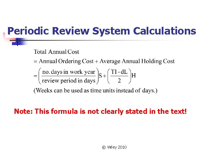
Periodic Review System Calculations Note: This formula is not clearly stated in the text! © Wiley 2010

Periodic Review (P) Model, Example 1: Your firm’s demand is normally distributed with mean 48/week and standard deviation 8. Lead time is 2 weeks, and the desired cycle service level is 94%. Initially, your review period is 1 week (every Friday you take inventory). Find the safety stock and the Target Inventory Level. [Ch. 12 #27. ] Safety Stock SS = z 94σRP+L z 94 =1. 55 Area =. 44 Stockout! Tail Area =. 06 Area left of y-axis =. 50 Safety Stock SS = (1. 55) (13. 86) = 21. 48 -> 22 0 © Wiley 2010 Z 94 = 1. 55 z

Periodic Review (P) Model, Example 1, continued: [Ch. 12 #27. ] We found Safety Stock SS = (1. 55) (13. 86) = 21. 48 -> 22 Next find the Target Inventory level (TI): TI = d(RP + L) + SS = (48) (1+2) + 22 = 166 units Follow-up: if you have 100 units on hand (OH =100), Order quantity q = TI – OH = 66 © Wiley 2010

Periodic Review (P) Model, Example 1, extended: [Ch. 12 #27. ] Suppose that the unit order cost is S = $25 and the unit holding cost is H=$2. Assuming 50 working weeks in the year, what is the total annual cost of inventory? = $50 + $70 = $120 © Wiley 2010

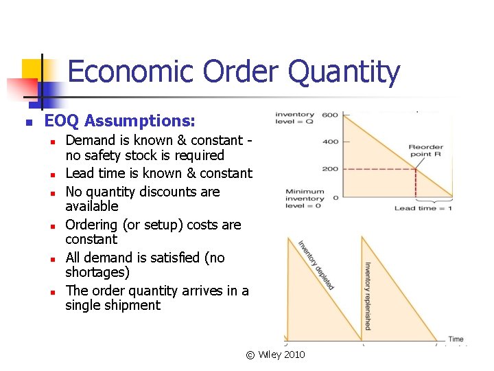
Economic Order Quantity n EOQ Assumptions: n n n Demand is known & constant no safety stock is required Lead time is known & constant No quantity discounts are available Ordering (or setup) costs are constant All demand is satisfied (no shortages) The order quantity arrives in a single shipment © Wiley 2010

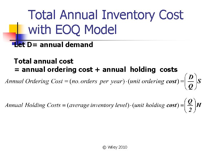
Total Annual Inventory Cost with EOQ Model Let D= annual demand Total annual cost = annual ordering cost + annual holding costs © Wiley 2010

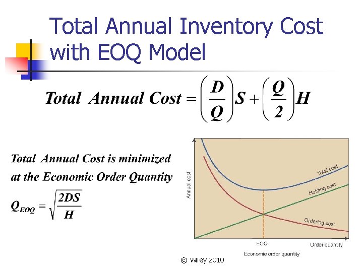
Total Annual Inventory Cost with EOQ Model © Wiley 2010

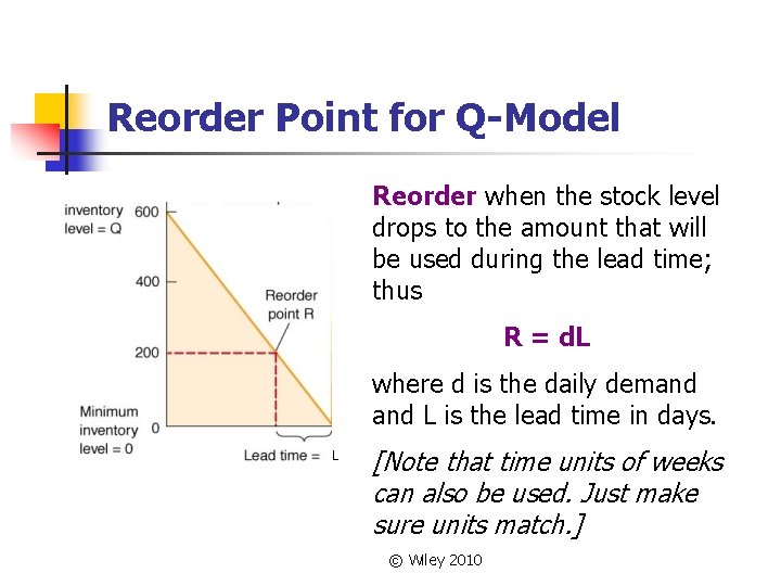
Reorder Point for Q-Model Reorder when the stock level drops to the amount that will be used during the lead time; thus R = d. L where d is the daily demand L is the lead time in days. L [Note that time units of weeks can also be used. Just make sure units match. ] © Wiley 2010

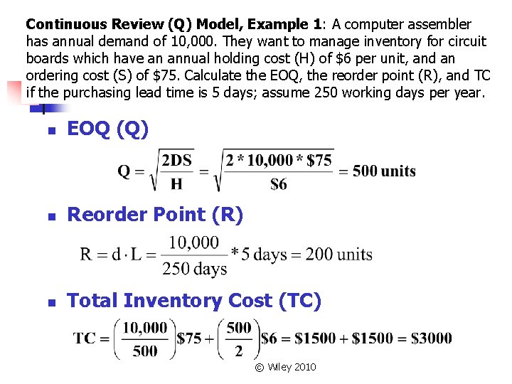
Continuous Review (Q) Model, Example 1: A computer assembler has annual demand of 10, 000. They want to manage inventory for circuit boards which have an annual holding cost (H) of $6 per unit, and an ordering cost (S) of $75. Calculate the EOQ, the reorder point (R), and TC if the purchasing lead time is 5 days; assume 250 working days per year. n EOQ (Q) n Reorder Point (R) n Total Inventory Cost (TC) © Wiley 2010

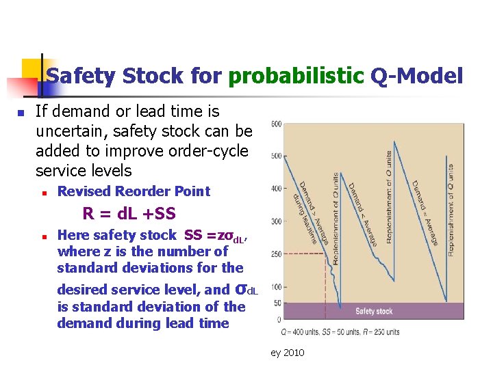
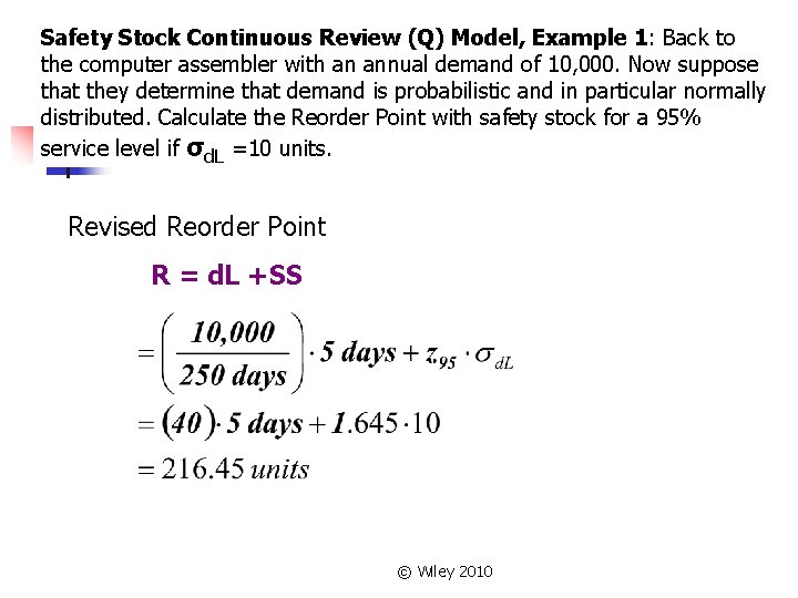
Safety Stock for probabilistic Q-Model n If demand or lead time is uncertain, safety stock can be added to improve order-cycle service levels n Revised Reorder Point R = d. L +SS n Here safety stock SS =zσd. L, where z is the number of standard deviations for the desired service level, and σd. L is standard deviation of the demand during lead time © Wiley 2010

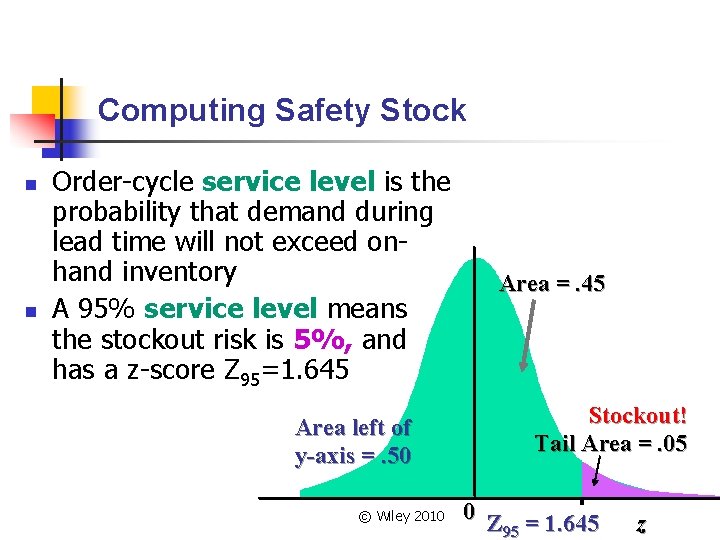
Computing Safety Stock n n Order-cycle service level is the probability that demand during lead time will not exceed onhand inventory A 95% service level means the stockout risk is 5%, and has a z-score Z 95=1. 645 Area left of y-axis =. 50 © Wiley 2010 Area =. 45 Stockout! Tail Area =. 05 0 Z 95 = 1. 645 z

Safety Stock Continuous Review (Q) Model, Example 1: Back to the computer assembler with an annual demand of 10, 000. Now suppose that they determine that demand is probabilistic and in particular normally distributed. Calculate the Reorder Point with safety stock for a 95% service level if σd. L =10 units. Revised Reorder Point R = d. L +SS © Wiley 2010

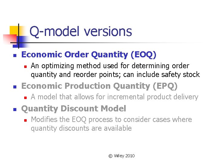
Q-model versions n Economic Order Quantity (EOQ) n n Economic Production Quantity (EPQ) n n An optimizing method used for determining order quantity and reorder points; can include safety stock A model that allows for incremental product delivery Quantity Discount Model n Modifies the EOQ process to consider cases where quantity discounts are available © Wiley 2010

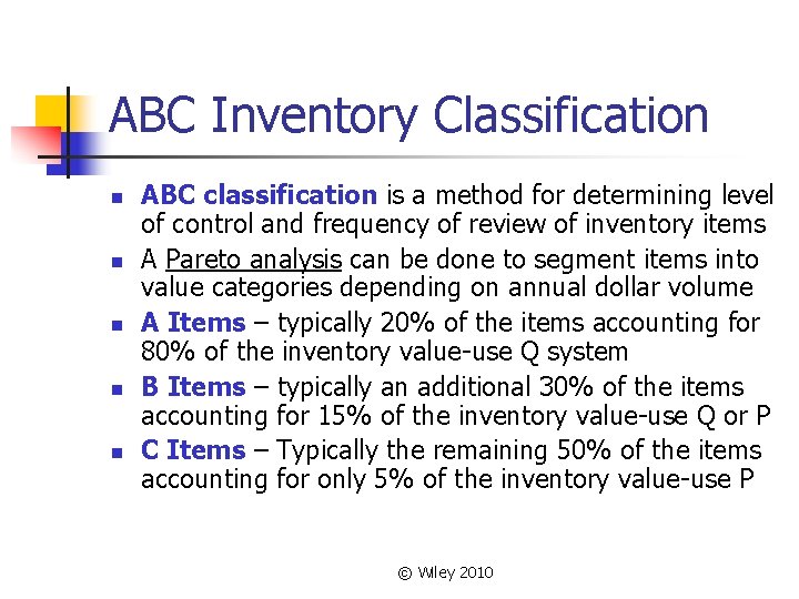
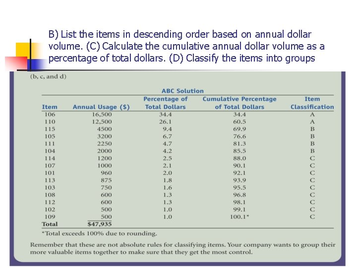
ABC Inventory Classification n n ABC classification is a method for determining level of control and frequency of review of inventory items A Pareto analysis can be done to segment items into value categories depending on annual dollar volume A Items – typically 20% of the items accounting for 80% of the inventory value-use Q system B Items – typically an additional 30% of the items accounting for 15% of the inventory value-use Q or P C Items – Typically the remaining 50% of the items accounting for only 5% of the inventory value-use P © Wiley 2010

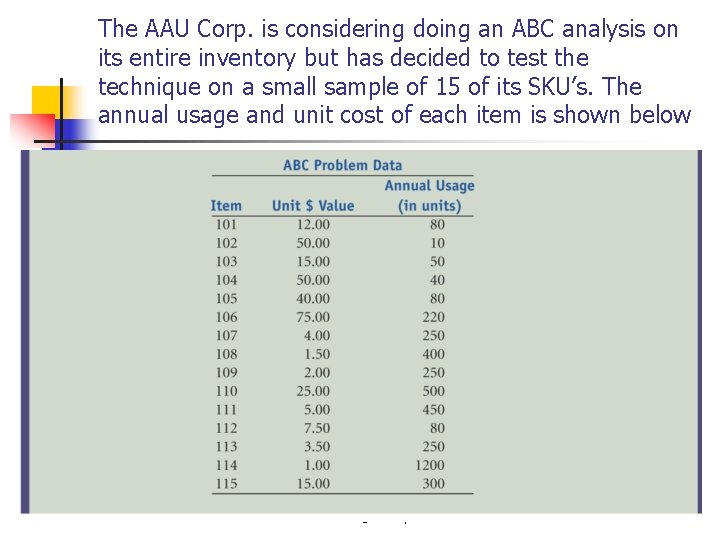
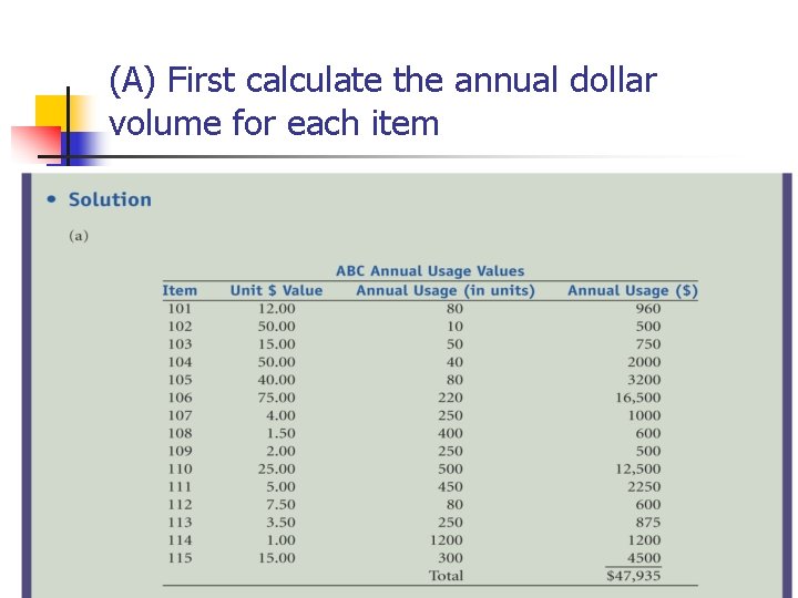
The AAU Corp. is considering doing an ABC analysis on its entire inventory but has decided to test the technique on a small sample of 15 of its SKU’s. The annual usage and unit cost of each item is shown below © Wiley 2010

(A) First calculate the annual dollar volume for each item © Wiley 2010

B) List the items in descending order based on annual dollar volume. (C) Calculate the cumulative annual dollar volume as a percentage of total dollars. (D) Classify the items into groups © Wiley 2010

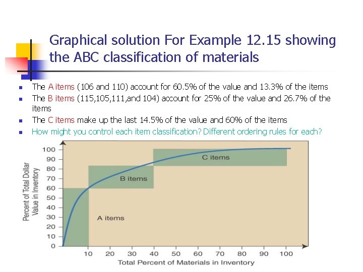
Graphical solution For Example 12. 15 showing the ABC classification of materials n n The A items (106 and 110) account for 60. 5% of the value and 13. 3% of the items The B items (115, 105, 111, and 104) account for 25% of the value and 26. 7% of the items The C items make up the last 14. 5% of the value and 60% of the items How might you control each item classification? Different ordering rules for each? © Wiley 2010

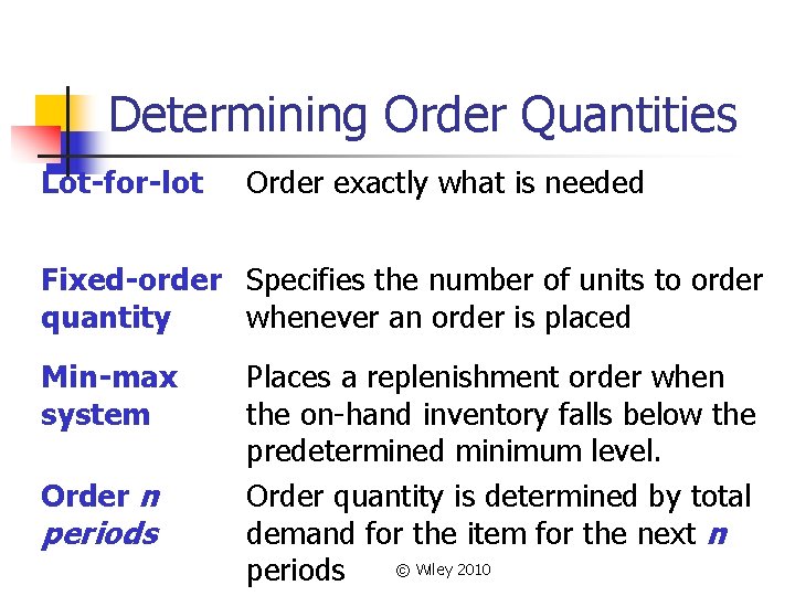
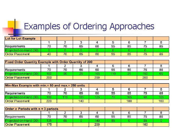
Determining Order Quantities Lot-for-lot Order exactly what is needed Fixed-order Specifies the number of units to order quantity whenever an order is placed Min-max system Order n periods Places a replenishment order when the on-hand inventory falls below the predetermined minimum level. Order quantity is determined by total demand for the item for the next n © Wiley 2010 periods

Examples of Ordering Approaches © Wiley 2010

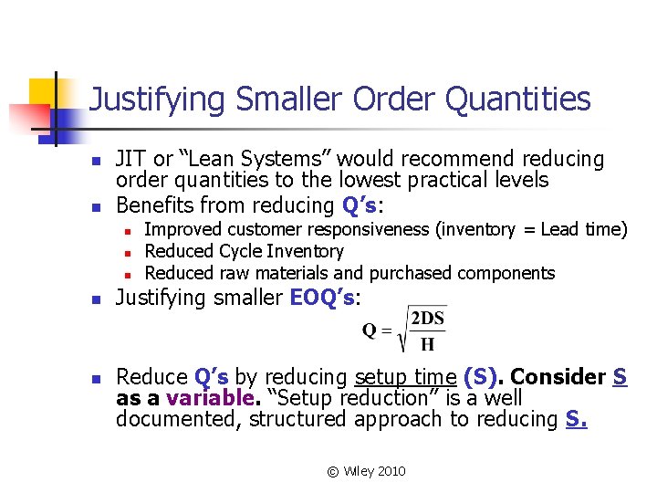
Justifying Smaller Order Quantities n n JIT or “Lean Systems” would recommend reducing order quantities to the lowest practical levels Benefits from reducing Q’s: n n n Improved customer responsiveness (inventory = Lead time) Reduced Cycle Inventory Reduced raw materials and purchased components Justifying smaller EOQ’s: Reduce Q’s by reducing setup time (S). Consider S as a variable. “Setup reduction” is a well documented, structured approach to reducing S. © Wiley 2010

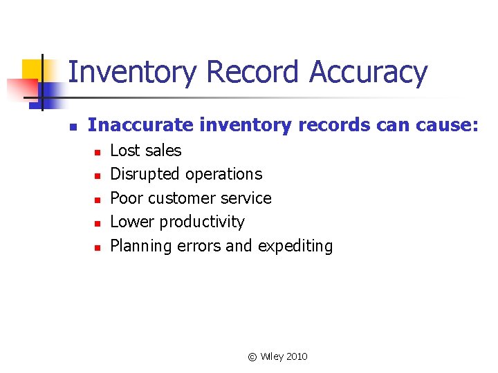
Inventory Record Accuracy n Inaccurate inventory records can cause: n n n Lost sales Disrupted operations Poor customer service Lower productivity Planning errors and expediting © Wiley 2010

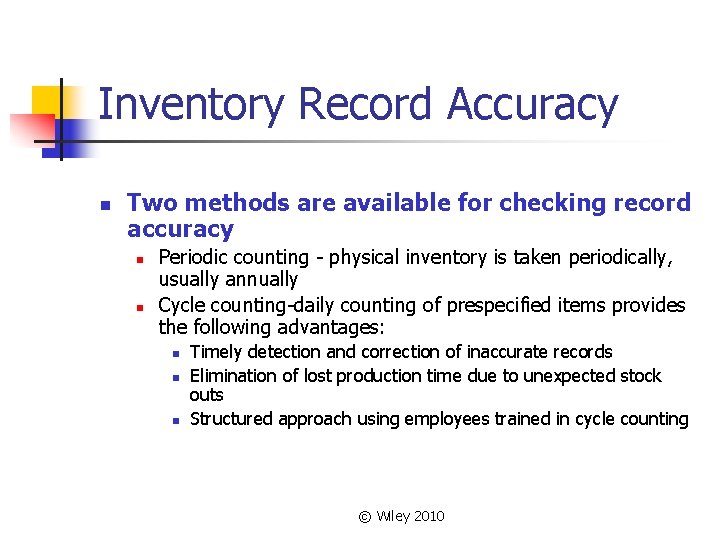
Inventory Record Accuracy n Two methods are available for checking record accuracy n n Periodic counting - physical inventory is taken periodically, usually annually Cycle counting-daily counting of prespecified items provides the following advantages: n n n Timely detection and correction of inaccurate records Elimination of lost production time due to unexpected stock outs Structured approach using employees trained in cycle counting © Wiley 2010

Ultimate Objective of Inventory Management n n Provide desired customer service level Customer service is the ability to satisfy customer requirements n n Percentage of orders shipped on schedule Percentage of line items shipped on schedule Percentage of dollar volume shipped on schedule Idle time due to material and component shortages © Wiley 2010

Customer Service Level Examples n Percentage of Orders Shipped on Schedule n n n Percentage of Line Items Shipped on Schedule n n n Good measure if orders have similar value. Does not capture value. If one company represents 50% of your business but only 5% of your orders, 95% on schedule could represent only 50% of value Recognizes that not all orders are equal, but does not capture $ value of orders. More expensive to measure. Ok for finished goods. A 90% service level might mean shipping 225 items out of the total 250 line items totaled from 20 orders scheduled Percentage Of Dollar Volume Shipped on Schedule n Recognizes the differences in orders in terms of both line items and $ value © Wiley 2010

Inventory Management Across the Organization n Inventory management policies affect functional areas throughout n n n Accounting is concerned of the cost implications of inventory Marketing is concerned as stocking decision affect the level of customer service Information Systems is involved to tack and control inventory records © Wiley 2010

Chapter 12 Highlights n Raw materials, purchased components, workin-process, finished goods, distribution inventory and maintenance, repair and operating supplies are all types of inventory. Inventories have several uses: anticipation inventory is built before it is needed; fluctuation stock provides a cushion; cycle stock is a result of the company’s ordering quantity; transportation inventory includes items in transit; speculative inventory is a buildup to protect against some future event and MRO inventory supports daily operations © Wiley 2010

Chapter 12 Highlights n n The objectives of inventory management are to provide the desired level of customer service, to allow cost-efficient operations, and to minimize inventory investment. Customer service can be measured in several ways, including as a percentage of orders shipped on schedule, a percentage of line items shipped on schedule, a percentage of dollar volume shipped on schedule, or idle time due to material and component shortages. Cost-efficient operations are achieved by using inventory as buffer stocks allowing a stable year-round workforce, and spreading the setup cost over a larger number of Inventory performance is measured by turns/supply. Inventory costs include item cost, holding cost, ordering cost, and shortage cost. © Wiley 2010

Chapter 12 Highlights n n (continued) Inventory investment is measured in inventory turnover and/or level of supply. Inventory performance is calculated as inventory turnover or weeks, days, or hours of supply. Relevant inventory costs include items costs, holding costs, and shortage costs. Holding costs include capital costs, storage costs, and risk costs. Ordering costs are fixed costs for placing an order or performing a setup. Shortage costs included costs related to additional paperwork, additional shipping expense, and the intangible cost of lost customer goodwill. © Wiley 2010

Chapter 12 Highlights n n (continued) Lot-for-lot, fixed-order quantity, min-max systems, order n periods, periodic review systems, EOQ models, quantity discount models, and single-period models can be used to determine order quantities. Ordering decisions can be improved by analyzing total costs of an inventory policy. Total costs include ordering cost, holding cost, and material cost © Wiley 2010

Chapter 12 Highlights n n n (continued) Practical considerations can cause a company to not use the optimal order quantity, that is, minimum order requirements Smaller lot sizes give a company flexibility and shorter response times. The key to reducing order quantities is to reduce ordering or setup costs. Calculating the appropriate safety stock policy enables companies to satisfy their customer service objective at minimum costs. The desired customer service level determines the appropriate z value. © Wiley 2010

Chapter 12 Highlights n n n (continued) Inventory decisions about perishable products can be made using the single-period inventory model. The expected payoff is calculated to assist the quantity decision The ABC classification system allows a company to assign the appropriate level of control and frequency of review of an item based on its annual dollar volume Cycle counting is a method for maintaining accurate inventory records. Determining what and when to count are the major decisions © Wiley 2010

Chapter 12 Highlights n n n n (continued) Order Q’s can be determined by using L 4 L, fixed order Q’s, minmax, order n periods, quantity discounts, and single period systems. Ordering decisions can be improved by analyzing TC Smaller lot sizes increase flexibility and reduce response time. Safety stock can be added to reorder point calculations to meet desired service level z value. Inventory decisions about perishable products can be made by using the single-period inventory model. ABC analysis can be used to assign the appropriate level of control and review frequency based on the annual dollar volume of each item. Cycle counting of pre-specified items is an accepted method for maintaining inventory records © Wiley 2010